13.1: Adiabatic Invariants

Imagine a particle in one dimension oscillating back and forth in some potential. The potential doesn’t have to be harmonic, but it must be such as to trap the particle, which is executing periodic motion with period T. Now suppose we gradually change the potential, but keeping the particle trapped. That is, the potential depends on some parameter \(\lambda\), which we change gradually, meaning over a time much greater than the time of oscillation: \(T d \lambda / d t \ll \lambda\)

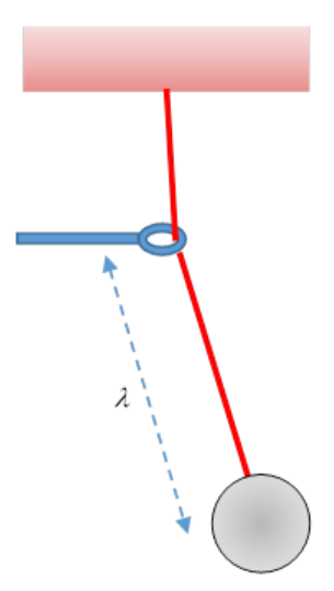
A crude demonstration is a simple pendulum with a string of variable length, for example one hanging from a fixed support, but the string passing through a small loop that can be moved vertically to change the effective length (Figure \(\PageIndex{1}\)).

Figure \(\PageIndex{1}\): Copy and Paste Caption here. (Copyright; author via source)

If \(λ\) were fixed, the system would have constant energy \(E\) and period \(T\). As λ is gradually changed from outside, there will be energy exchange in general, we’ll write the Hamiltonian \(H(q, p ; \lambda)\), the energy of the system will be \(E(\lambda)\) (Of course, \(E\) also depends on the initial energy before the variation began.) Remember now that from Hamilton’s equations \(d H / d t=\partial H / \partial t\) so during the variation

\begin{equation}\frac{d E}{d t}=\frac{\partial H}{\partial t}=\frac{\partial H}{\partial \lambda} \frac{d \lambda}{d t}\end{equation}

It’s clear from the diagram that the energy fed into the system as the ring moves slowly down varies throughout the cycle—for example, when the pendulum is close to vertically down, its energy will be almost unaffected by moving the ring.

Moving slowly down means \(\lambda\) varies very little in one cycle of the system, we can average over a cycle:

\begin{equation}\frac{d E}{d t}=\frac{\overline{\partial H}}{\partial \lambda} \frac{d \lambda}{d t}\end{equation}

where

\begin{equation}\frac{\partial H}{\partial \lambda}=\frac{1}{T} \int_{0}^{T} \frac{\partial H}{\partial \lambda} d t\end{equation}

Now Hamilton’s equation \(d q / d t=\partial H / \partial p\) means that we can replace \(d t\) with \(\frac{d q}{(\partial H / \partial p)_{\lambda}}\), so the time for going round one complete cycle is

\begin{equation}T=\int_{0}^{T} d t=\oint \frac{d q}{(\partial H / \partial p)_{\lambda}}\end{equation}

(This won’t integrate to zero, because on the return leg both \(d q \text { and } \dot{q}=(\partial H / \partial p)\) will be negative.)

Therefore, replacing \(d t \text { in } \int_{0}^{T}(\partial H / \partial \lambda)\) as well,

\begin{equation}\frac{\overline{d E}}{d t}=\frac{d \lambda}{d t} \frac{\oint \frac{(\partial H / \partial \lambda) d q}{\partial H / \partial p}}{\oint \frac{d q}{(\partial H / \partial p)_{\lambda}}}\end{equation}

Now, we assume \(λ, E\) are varying slowly enough that they are close to constant over one cycle, meaning that at a given point q on the circuit, the momentum can be written \(p=p(q ; E, \lambda), \text { regarding } E, \lambda\) as constant and independent parameters. (We can always adjust \(E \text { at fixed } \lambda \text { by giving the pendulum a little push!) }\)

If we now partially differentiate \(H(q, p, \lambda)=E \text { with respect to } \lambda, \text { keeping } E\) constant (appropriate infinitesimal pushes required!), we get, at point \(q\) on the circuit,

\begin{equation}\partial H / \partial \lambda+(\partial H / \partial p)(\partial p / \partial \lambda)=0, \text { or } \partial p(q, \lambda, E) / \partial \lambda=-\frac{\partial H / \partial \lambda}{\partial H / \partial p}\end{equation}

which is the integrand in the numerator of our expression for \(\frac{d E}{d t}, \text { so }\)

\begin{equation}\frac{\overline{d E}}{d t}=-\frac{d \lambda}{d t} \frac{\oint(\partial p / \partial \lambda)_{E} d q}{\oint(\partial p / \partial E)_{\lambda} d q}\end{equation}

In the denominator, we’ve replaced \(1 /(\partial H / \partial p)_{\lambda} \text { by }(\partial p / \partial E)_{\lambda}\)

Rearranging,

\begin{equation}
\oint\left[\left(\frac{\partial p}{\partial E}\right)_{\lambda} \frac{\overline{d E}}{d t}+\left(\frac{\partial p}{\partial \lambda}\right)_{E} \frac{d \lambda}{d t}\right] d q=0
\end{equation}

This can be written

\begin{equation}
\frac{\overline{d I}}{d t}=0, \quad \text { where } I=\frac{1}{2 \pi} \oint p(q, \lambda, E) d q
\end{equation}

\(I\) is an adiabatic invariant: That means it stays constant when the parameters of the system change gradually, even though the system’s energy changes.

Important! The partial derivative with respect to energy \(\partial I / \partial E\) determines the period of the motion:

\begin{equation}2 \pi \frac{\partial I}{\partial E}=\oint\left(\frac{\partial p}{\partial E}\right)_{\lambda} d q=\oint \frac{d q}{(\partial H / \partial p)_{\lambda}}=\oint \frac{d q}{\dot{q}}=T, \quad \text { or } \partial E / \partial I=\omega\end{equation}

(Note: here is another connection with quantum mechanics. If the system is connected to the outside world, for example if the orbiting particle is charged, as it usually is, and can therefore emit radiation, since in quantum mechanics successive action numbers \(I\) differ by integers, and the quantum of action is \(\hbar\), the energy radiated per quantum drop in action is \(\hbar \omega\). This is of course in the classical limit of high quantum numbers.)

Notice that \(I\) is the area of phase space enclosed by the integral,

\begin{equation}I=\frac{1}{2 \pi} \oint p d q=\iint \frac{d p d q}{2 \pi}\end{equation}

For the SHO, it’s easy to check from the area of the ellipse that \(I=E / \omega\)

Take

\begin{equation}H=(1 / 2 m)\left(p^{2}+m \omega^{2} q^{2}\right)\end{equation}

The phase space elliptical orbit has semi-axes with lengths \(\sqrt{2 m E}, \quad \sqrt{2 E / m \omega^{2}}\), so the area enclosed is \(\pi a b=2 \pi E / \omega\).

The bottom line is that as we gradually change the spring strength (or, for that matter, the mass) of an oscillator (not necessarily harmonic), the energy changes proportionally with the frequency.