14.2: The Ellipse

Squashed Circles and Gardeners

The simplest nontrivial planetary orbit is a circle: \(x^{2}+y^{2}=a^{2}\) is centered at the origin and has radius \(a\). An ellipse is a circle scaled (squashed) in one direction, so an ellipse centered at the origin with semimajor axis \(a\) and semiminor axis \(b<a\) has equation

\[\dfrac{x^{2}}{a^{2}}+\frac{y^{2}}{b^{2}}=1\]

in the standard notation, a circle of radius \(a\) scaled by a factor \(b/a\) in the \(y\) direction. (It’s usual to orient the larger axis along \(x\). )

A circle can also be defined as the set of points which are the same distance a from a given point, and an ellipse can be defined as the set of points such that the sum of the distances from two fixed points is a constant length (which must obviously be greater than the distance between the two points!). This is sometimes called the gardener’s definition: to set the outline of an elliptic flower bed in a lawn, a gardener would drive in two stakes, tie a loose string between them, then pull the string tight in all different directions to form the outline.

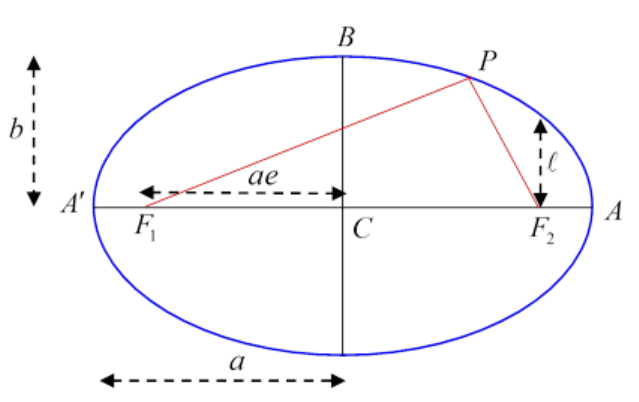
In the diagram, the stakes are at \(F_{1}, F_{2}\) the red lines are the string, \(P\) is an arbitrary point on the ellipse.

\(CA\) is called the semimajor axis length a, \(CB\) the semiminor axis, length \(b\).

\(F_{1}, F_{2}\) are called the foci (plural of focus).

Notice first that the string has to be of length \(2a\), because it must stretch along the major axis from \(F_{1} \text { to } A\) then back to \(F_{2}\) and for that configuration there’s a double length of string along \(F_{2} A \text { and a single length from } F_{1} \text { to } F_{2}\). But the length \(A^{\prime} F_{1} \text { is the same as } F_{2} A\), so the total length of string is the same as the total length \(A^{\prime} A=2 a\).

Suppose now we put \(P\) at \(B\). Since \(F_{1} B=B F_{2}\), and the string has length \(2 a, \text { the length } F_{1} B=a\)

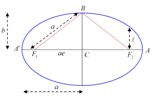
We get a useful result by applying Pythagoras’ theorem to the triangle \(F_{1} B C\)

\[\left(F_{1} C\right)^{2}=a^{2}-b^{2}\]

(We shall use this shortly.)

Evidently, for a circle, \(F_{1} C=0\)

Eccentricity

The eccentricity \(e\) of the ellipse is defined by

\[e=F_{1} C / a=\sqrt{1-(b / a)^{2}}, \quad \text { note } e<1\]

Eccentric just means off center, this is how far the focus is off the center of the ellipse, as a fraction of the semimajor axis. The eccentricity of a circle is zero. The eccentricity of a long thin ellipse is just below one.

\(F_{1} \text { and } F_{2}\) on the diagram are called the foci of the ellipse (plural of focus) because if a point source of light is placed at \(F_{1}\), and the ellipse is a mirror, it will reflect—and therefore focus—all the light to \(F_{2}\).

Equivalence of the Two Definitions

We need to verify, of course, that this gardener’s definition of the ellipse is equivalent to the squashed circle definition. From the diagram, the total string length

\[2 a=F_{1} P+P F_{2}=\sqrt{(x+a e)^{2}+y^{2}}+\sqrt{(x-a e)^{2}+y^{2}}\]

and squaring both sides of

\[2 a-\sqrt{(x+a e)^{2}+y^{2}}=\sqrt{(x-a e)^{2}+y^{2}}\]

then rearranging to have the residual square root by itself on the left-hand side, then squaring again,

\[(x+a e)^{2}+y^{2}=(a+e x)^{2}\]

\(\text { from which, using } e^{2}=1-\left(b^{2} / a^{2}\right), \text { we find } x^{2} / a^{2}+y^{2} / b^{2}=1\)

Ellipse in Polar Coordinates

In fact, in analyzing planetary motion, it is more natural to take the origin of coordinates at the center of the Sun rather than the center of the elliptical orbit.

It is also more convenient to take \((r,\theta)\) coordinates instead of \((x,y)\) coordinates, because the strength of the gravitational force depends only on \(r\). Therefore, the relevant equation describing a planetary orbit is the \((r,\theta)\) equation with the origin at one focus, here we follow the standard usage and choose the origin at \(F_{2}\).

For an ellipse of semi major axis \(a\) and eccentricity \(e\) the equation is:

\[\frac{a\left(1-e^{2}\right)}{r}=1+e \cos \theta\]

This is also often written

\[\frac{\ell}{r}=1+e \cos \theta\]

where \(ℓ\) is the semi-latus rectum, the perpendicular distance from a focus to the curve \((\operatorname{so} \theta=\pi / 2)\), see the diagram below: but notice again that this equation has \(F_{2} \text { as its origin! (For } \left.\theta<\pi / 2, r<\ell .\right)\)

(It’s easy to prove \(\ell=a\left(1-e^{2}\right)\) using Pythagoras’ theorem, \((2 a-\ell)^{2}=(2 a e)^{2}+\ell^{2}\)

The directrix: writing \(r \cos \theta=x\), the equation for the ellipse can also be written as

\[r=a\left(1-e^{2}\right)-e x=e\left(x_{0}-x\right)\]

where \(x_{0}=(a / e)-a e\) (the origin x=0 being the focus).

The line \(x=x_{0}\) is called the directrix.

For any point on the ellipse, its distance from the focus is e times its distance from the directrix.

Deriving the Polar Equation from the Cartesian Equation

Note first that (following standard practice) coordinates \((x,y)\) and \((r,\θ)\) have different origins!

Writing \(x=a e+r \cos \theta, y=r \sin \theta\) in the Cartesian equation,

\[\frac{(a e+r \cos \theta)^{2}}{a^{2}}+\frac{(r \sin \theta)^{2}}{b^{2}}=1\]

that is, with slight rearrangement,

\[r^{2}\left(\frac{\cos ^{2} \theta}{a^{2}}+\frac{\sin ^{2} \theta}{b^{2}}\right)+r \frac{2 e \cos \theta}{a}-\left(1-e^{2}\right)=0\]

This is a quadratic equation for \(r\) and can be solved in the usual fashion, but looking at the coefficients, it’s evidently a little easier to solve the corresponding quadratic for \(u=1 / r\)

The solution is:

\[\frac{1}{r}=u=\frac{e \cos \theta}{a\left(1-e^{2}\right)} \pm \frac{1}{a\left(1-e^{2}\right)}\]

from which

\[\frac{a\left(1-e^{2}\right)}{r}=\frac{\ell}{r}=1+e \cos \theta\]

where we drop the other root because it gives negative \(r\), for example for \(\theta=\pi / 2\). This establishes the equivalence of the two equations.