16.4: Analyzing Inverse-Square Repulsive Scattering- Kepler Again

To make further progress, we must calculate \(b(\chi)\), or equivalently \(\chi(b)\): what is the angle of scattering, the angle between the outgoing velocity and the ingoing velocity, for a given impact parameter? \(\chi\) will of course also depend on the strength of the repulsion, and the ingoing particle energy.

Recall our equation for Kepler orbits:

\begin{equation}\frac{d^{2} u}{d \theta^{2}}+u=\frac{G M m^{2}}{L^{2}}\end{equation}

Let’s now switch from gravitational scattering with an attractive force \(G M m / r^{2}\) to an electrical repulsive force between two charges \(Z_{1} e, Z_{2} e\), force strength \(\frac{1}{4 \pi \varepsilon_{0}} \frac{Z_{1} Z_{2} e^{2}}{r^{2}}=\frac{k}{r^{2}}\), say. Since this is repulsive, the sign will change in the radial acceleration equation,

\begin{equation}\frac{d^{2} u}{d \theta^{2}}+u=-\frac{k m}{L^{2}}\end{equation}

Also, we want the scattering parameterized in terms of the impact parameter b and the incoming speed \(v_{\infty}\), so putting \(L=m v_{\infty} b\) this is

\begin{equation}\frac{d^{2} u}{d \theta^{2}}+u=-\frac{k}{m b^{2} v_{\infty}^{2}}\end{equation}

So just as with the Kepler problem, the orbit is given by

\begin{equation}\frac{1}{r}=u=-\frac{k}{m b^{2} v_{\infty}^{2}}+C \cos \left(\theta-\theta_{0}\right)=-\kappa+C \cos \left(\theta-\theta_{0}\right), \text { say. }\end{equation}

From the lecture on Orbital Mathematics, the polar equation for the left hyperbola branch relative to the external (right) focus is

\begin{equation}\mathrm{l} / r=-e \cos \theta-1\end{equation}

this is a branch symmetric about the \(x\)-axis:

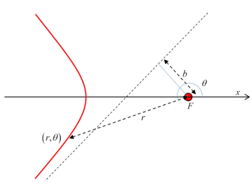
But we want the incoming branch to be parallel to the axis, which we do by suitable choice of \(\theta_{0}\). In other words, we rotate the hyperbola clockwise through half the angle between its asymptotes, keeping the scattering center (right-hand focus) fixed.

From the lecture on orbital mathematics (last page), the perpendicular distance from the focus to the asymptote is the hyperbola parameter \(b!\). Presumably, this is why we use \(b\) for the impact parameter. Hence the particle goes in a hyperbolic path with parameters \(e / \mathrm{l}=-C, \quad 1 / \mathrm{l}=\kappa\). This is not enough information to fix the path uniquely: we’ve only fed in the angular momentum \(m b v_{\infty}\) not the energy, so this is a family of paths having different impact parameters but the same angular momentum .

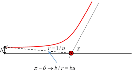
We can, however, fix the path uniquely by equating the leading order correction to the incoming zeroth order straight path: the particle is coming in parallel to the \(x\)-axis far away to the left, perpendicular distance \(b\) from the axis, that is, from the line \(\theta=\pi\). So, going back to that pre-scattering time,

\begin{equation}u \rightarrow 0, \quad \pi-\theta \rightarrow b / r=b u\end{equation}

and in this small \(u\) limit,

\begin{equation}u=C \cos \left(\pi-b u-\theta_{0}\right)-\kappa \cong C \cos \left(\pi-\theta_{0}\right)-\kappa+b C u \sin \left(\pi-\theta_{0}\right)\end{equation}

Matching the zeroth order and the first order terms

\begin{equation}C \cos \left(\pi-\theta_{0}\right)=\kappa, \quad u=b C u \sin \left(\pi-\theta_{0}\right)\end{equation}

eliminates \(C\) and fixes the angle \(\theta_{0}\), which is the angle the hyperbola had to be rotated through to align the asymptote with the negative \(x\)-axis, and therefore half the angle between the asymptotes, which would be \(\pi\) minus the angle of scattering \(\chi\) (see the earlier diagram),

\begin{equation}\tan \left(\pi-\theta_{0}\right)=-\tan \theta_{0}=\frac{1}{b \kappa}=\frac{m b v_{\infty}^{2}}{k}\end{equation}

\begin{equation}\chi=\pi-2 \cot ^{-1} b \kappa=2 \tan ^{-1} b \kappa\end{equation}

So this is the scattering angle in terms of the impact parameter \(b\), that is, in the diagram above

\begin{equation}\chi(b)=2 \tan ^{-1}\left(\frac{k}{m b v_{\infty}^{2}}\right)\end{equation}

Equivalently,

\begin{equation}
b=\frac{k}{m v_{\infty}^{2}} \cot \frac{\chi}{2}, \text { so } d b=\frac{k}{2 m v_{\infty}^{2}} \operatorname{cosec}^{2} \frac{\chi}{2} d \chi
\end{equation}

and the incremental cross sectional area

\begin{equation}
d \sigma=2 \pi b d b=\pi\left(\frac{k}{m v_{\infty}^{2}}\right)^{2} \operatorname{cosec}^{2} \frac{1}{2} \chi \cot \frac{1}{2} \chi d \chi=\pi\left(\frac{k}{m v_{\infty}^{2}}\right)^{2} \frac{\cos \frac{1}{2} \chi}{\sin ^{3} \frac{1}{2} \chi} d \chi=\left(\frac{k}{2 m v_{\infty}^{2}}\right)^{2} \frac{1}{\sin ^{4} \frac{1}{2} \chi} d \Omega
\end{equation}

This is Rutherford’s formula: the incremental cross section for scattering into an incremental solid angle, the differential cross section

\begin{equation}
\frac{d \sigma}{d \Omega}=\left(\frac{k}{2 m v_{\infty}^{2}}\right)^{2} \frac{1}{\sin ^{4} \frac{1}{2} \chi}
\end{equation}

\(\begin{equation}
\text { (Recall } k=\frac{1}{4 \pi \varepsilon_{0}} Z_{1} Z_{2} e^{2} \text { in MKS units. })
\end{equation}\)