22.5: Nonlinear Case - Landau’s Analysis

The equation of motion is:

\[\ddot{x}+2 \lambda \dot{x}+\omega_{0}^{2} x=(f / m) \cos \gamma t-\beta x^{3}\]

We established earlier that the nonlinear quartic term brings in a correction to the oscillator’s frequency that depends on the amplitude \(b\):

\[\omega=\omega_{0}+\frac{3 \beta b^{2}}{8 \omega_{0}}=\omega_{0}+\kappa b^{2}\]

in Landau’s notation \(\kappa=3 \beta / 8 \omega_{0}\),

The equation for the amplitude in the linear case (from the previous section) was, with \(\varepsilon=\gamma-\omega_{0}\),

\[b^{2}\left(\varepsilon^{2}+\lambda^{2}\right)=\frac{f^{2}}{4 m^{2} \omega_{0}^{2}}\]

For the nonlinear case, the maximum amplitude will clearly be at the true (amplitude dependent!) resonance frequency \(\omega(b)=\omega_{0}+\kappa b^{2} \text { so with } \varepsilon=\gamma-\omega_{0}\) before, we now have a cubic equation for \(b^{2}\):

\[b^{2}\left(\left(\varepsilon-\kappa b^{2}\right)^{2}+\lambda^{2}\right)=\frac{f^{2}}{4 m^{2} \omega_{0}^{2}}\]

Note that for small driving force \(f \ll 2 m \omega_{0} \lambda, b\) is small (\(b_{\max }^{2} \approx f^{2} / 4 m^{2} \omega_{0}^{2} \lambda^{2}\)) but the center of the peak has shifted slightly upwards, to \(\varepsilon=\kappa b^{2}, \text { that is, at a driving frequency } \gamma=\omega_{0}+\kappa b^{2}\). The cubic equation for \(b^{2}\) has only this one real solution.

However, as the driving force is increased, the coefficients of the cubic equation change and at a critical force \(f_{k}\) two more real roots appear.

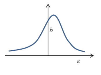
\(\text { The } b, \varepsilon \text { curve for driving force above } f_{k} \text { looks like: }\)

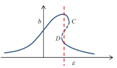
So what’s going on here? For a range of frequencies, including the vertical dashed red line in the figure, there appear to be three possible amplitudes of steady oscillation at one frequency. However, it turns out that the middle one is unstable, so will exponentially deviate, going to one of the other two, both of which are stable.

If the oscillator is being driven at \(\omega_{0}\), and the driving frequency is gradually increased, the amplitude will follow the upper curve to the point C , then drop discontinuously to the lower curve. Further frequency increase (with the same strength driving force, of course) will give diminishing amplitude of oscillation just as happens for the ordinary simple harmonic oscillator on going away from the resonant frequency.

If the frequency is now gradually lowered, the amplitude gradually will increase to point D, where it will jump discontinuously to the upper curve. The overall response to driving frequency is sometimes called hysteresis, by analogy with the response of a magnetic material to a varying imposed external field.

\(\begin{aligned}&\text { To put in some numbers, the maximum amplitude for any of these curves is when } \quad d b / d \varepsilon=0, \text { that is, }\\&\text { at } \varepsilon=\kappa b^{2}, \text { or }\end{aligned}\)

\[b_{\max }=f / 2 m \omega_{0} \lambda\]

the same result as for small oscillations.

To find the critical value of the driving force for which the multiple solutions appear, in the graph above that’s when C, D coincide. That is, \(d b / d \varepsilon=\infty\) has coincident roots.

Differentiating the equation \(b(\varepsilon)\) for amplitude as a function of frequency (and of course this is at constant driving force \(f\))

\[\frac{d b}{d \varepsilon}=-\frac{-\varepsilon b+\kappa b^{2}}{\varepsilon^{2}+\lambda^{2}-4 \kappa \varepsilon b^{2}+3 \kappa^{2} b^{4}}\]

C,D coincide when the discriminant in the denominator quadratic is zero, that is, at \(\kappa^{2} b^{4}=\lambda^{2}\) where \(\varepsilon=2 \kappa b^{2}\)

Putting these values into the equation for \(b(\varepsilon)\) as a function of driving force f, the critical driving force is

\[f_{\kappa}^{2}=\frac{8 m^{2} \omega_{0}^{2} \lambda^{3}}{|\kappa|}\]

Numerical Applet Results

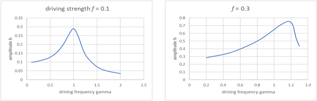
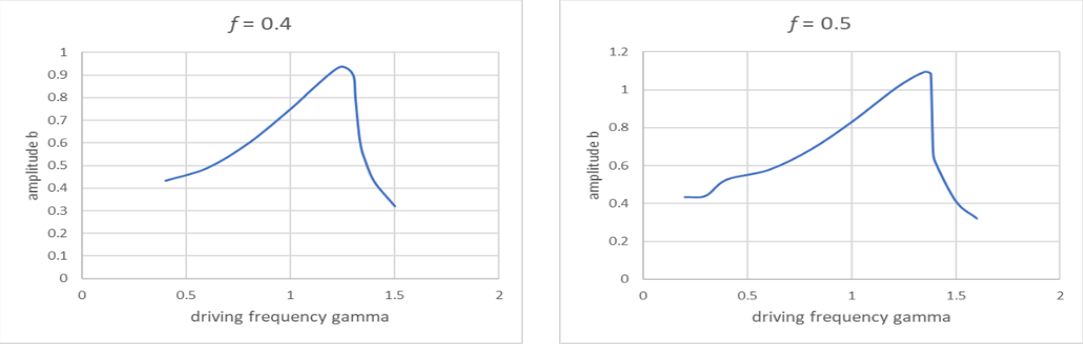
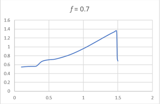
The results above are all from Landau’s book, and are semiquantitative. They can easily be checked using our online applet, which is accurate to one percent or better. The curves below are plotted from applet results, and certainly exhibit the behavior predicted by Landau.

These plots are for \(\omega_{0}^{2}=m=\beta=1, \alpha=0,2 \lambda=0.34\)

\(\begin{aligned}&\text { For these values, Landau's } f_{k} \text { is approximately } 0.3 . \text { Ours looks a bit more. Note for } f=0.3, \text { we show }\\
&\kappa b^{2}=0.38 \cdot(0.75)^{2}=0.21, \text { close to graph peak. }\end{aligned}\)