6.7: Applications to unconstrained systems

Although most dynamical systems involve constrained motion, it is useful to consider examples of systems subject to conservative forces with no constraints . For no constraints, the Lagrange-Euler equations \((6.6.1)\) simplify to \(\Lambda _{j}L=0\) where \(j=1,2,..n,\) and the transformation to generalized coordinates is of no consequence.

Example \(\PageIndex{1}\): Motion of a free particle, \(U=0\)

The Lagrangian in cartesian coordinates is \(L= \frac{1}{2}m(\dot{x}^{2}+\dot{y}^{2}+\dot{z}^{2}).\) Then

\[\begin{aligned} \frac{\partial L}{\partial \dot{x}} &= m\dot{x} \\[4pt] \frac{\partial L}{\partial \dot{y}} &= m\dot{y} \\[4pt] \frac{\partial L}{\partial \dot{z}} &= m\dot{z} \\[4pt] \frac{\partial L}{\partial x} &= \frac{\partial L}{\partial y}=\frac{ \partial L}{\partial z}=0\end{aligned}\]

Insert these in the Lagrange equation gives

\[\begin{align*} \Lambda _{x}L &= \frac{d}{dt}\frac{\partial L}{\partial \dot{x}}-\frac{\partial L}{\partial x} \\[4pt] &=\frac{d}{dt}m\dot{x}-0=0 \end{align*}\]

Thus

\[\begin{align*} \mathit{\ }p_{x} &= m\dot{x}=constant \\[4pt] p_{y} &= m\dot{y}=constant \\[4pt] \mathit{\ }p_{z} &= m\dot{z}=constant\end{align*}\]

That is, this shows that the linear momentum is conserved if \(U\) is a constant, that is, no forces apply. Note that momentum conservation has been derived without any direct reference to forces.

Example \(\PageIndex{2}\): Motion in a uniform gravitational field

Figure \(\PageIndex{1}\): Motion in a gravitational field

Consider the motion is in the \(x-y\) plane. The kinetic energy \(T= \frac{1}{2}m\left( \overset{.}{x}^{2}+\overset{.}{y}^{2}\right)\) while the potential energy is \(U=mgy\) where \(U(y=0)=0.\) Thus

\[L=\frac{1}{2}m\left( \overset{.}{x}^{2}+\overset{.}{y}^{2}\right) -mgy \nonumber\]

Using the Lagrange equation for the \(x\) coordinate gives

\[\begin{align*} \Lambda _{x}L &= \frac{d}{dt}\frac{\partial L}{\partial \overset{.}{x}}-\frac{ \partial L}{\partial x} \\[4pt] &=\frac{d}{dt}m\overset{.}{x}-0 \\[4pt] &=0 \end{align*}\]

Thus the horizontal momentum \(m\dot{x}\) is conserved and \(\overset{..}{x}=0.\) The \(y\) coordinate gives

\[ \begin{align*} \Lambda _{y}L &= \frac{d}{dt}\frac{\partial L}{\partial \overset{.}{y}}-\frac{ \partial L}{\partial y} \\[4pt] &=\frac{d}{dt}m\overset{.}{y}+mg \\[4pt] &=0 \end{align*}\]

Thus the Lagrangian produces the same results as derived using Newton’s Laws of Motion.

\[\ddot{x}=0 \nonumber\]

\[y=-g \nonumber\]

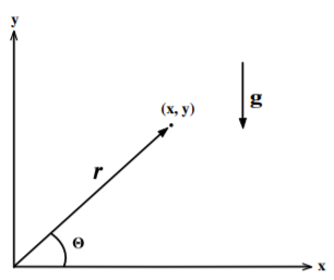
The importance of selecting the most convenient generalized coordinates is nicely illustrated by trying to solve this problem using polar coordinates \(r,\theta ,\) where \(r\) is radial distance and \(\theta\) the elevation angle from the \(x\) axis as shown in the adjacent figure. Then

\[T=\frac{1}{2}m\overset{.}{r}^{2}+\frac{1}{2}m\left( r\overset{.}{\theta } \right) ^{2} \nonumber\]

\[U=mgr\sin \theta \nonumber \]

Thus

\[L=\frac{1}{2}m\overset{.}{r}^{2}+\frac{1}{2}m\left( r\dot{\theta}\right) ^{2}-mgr\sin \theta \nonumber\]

\(\Lambda _{r}L=0\) for the \(r\) coordinate

\[r\dot{\theta}^{2}-g\sin \theta -\ddot{r}=0 \nonumber\]

\(\Lambda _{\theta }L=0\) for the \(\theta\) coordinate

\[-gr\cos \theta -2r\dot{r}\dot{\theta}-r^{2}\ddot{\theta}=0 \nonumber\]

These equations written in polar coordinates are more complicated than the result expressed in Cartesian coordinates. This is because the potential energy depends directly on the \(y\) coordinate, whereas it is a function of both \(r,\theta .\) This illustrates the freedom for using different generalized coordinates, plus the importance of choosing a sensible set of generalized coordinates.

Example \(\PageIndex{3}\): Central forces

Consider a mass \(m\) moving under the influence of a spherically-symmetric, conservative, attractive, inverse-square force. The potential then is

\[U=- \frac{k}{r} \nonumber\]

It is natural to express the Lagrangian in spherical coordinates for this system. That is,

\[L=\frac{1}{2}m\dot{r}^{2}+\frac{1}{2}m\left( r\dot{\theta}\right) ^{2}+\frac{ 1}{2}m(r\sin \theta \dot{\phi})^{2}+\frac{k}{r} \nonumber\]

\(\Lambda _{r}L=0\) for the \(r\) coordinate gives \[m\ddot{r}-mr[\dot{\theta}^{2}+\sin ^{2}\theta \dot{\phi}^{2}]=\frac{k}{r^{2}} \nonumber\]

where the \(mr\sin ^{2}\theta \dot{\phi}^{2}\) term comes from the centripetal acceleration.

\(\Lambda _{\phi }L=0\) for the \(\phi\) coordinate gives

\[\frac{d}{dt}\left( mr^{2}\sin ^{2}\theta \dot{\phi}\right) =0 \nonumber\]

This implies that the derivative of the angular momentum about the \(\phi\) axis, \(\dot{p}_{\phi }=0\) and thus \(p_{\phi }= mr^{2}\sin ^{2}\theta \dot{\phi}\) is a constant of motion.

\(\Lambda _{\theta }L=0\) for the \(\theta\) coordinate gives

\[\frac{d}{dt}(mr^{2}\dot{\theta})-mr^{2}\sin \theta \cos \theta \dot{\phi} ^{2}=0 \nonumber\]

That is, \[\dot{p}_{\theta }=mr^{2}\sin \theta \cos \theta \dot{\phi}^{2}=\frac{p_{\phi }^{2}\cos \theta }{2mr^{2}\sin ^{3}\theta } \nonumber\]

Note that \(p_{\theta }\) is a constant of motion if \(p_{\phi }=0\) and only the radial coordinate is influenced by the radial form of the central potential.