9.2: Hamilton's Principle of Stationary Action

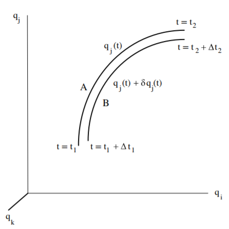
Hamilton’s crowning achievement was his use of the general form of Hamilton’s principle of stationary action $S$, equation $(9.1.2)$, to derive both Lagrangian mechanics, and Hamiltonian mechanics. Consider the action $S_{A}$ for the extremum path of a system in configuration space, that is, along path $A$ for $j=1,2,\dots ,n$ coordinates $q_{j}(t_{i})$ at initial time $t_{i}$ to $q_{j}(t_{f})$ at a final time $t_{f}$ as shown in Figure $\PageIndex{1}$.

Figure $\PageIndex{1}$: Extremum path A, plus the neighboring path B, shown in configuration space.

Then the action $S_{A}$ is given by

$$S_{A}=\int_{t_{i}}^{t_{f}}L(\mathbf{q}(t)\mathbf{, \dot{q}}(t)\mathbf{,}t)dt \label{9.3}$$

As used in chapter $5.2,$ a family of neighboring paths is defined by adding an infinitessimal fraction $\epsilon$ of a continuous, well-behaved neighboring function $\eta _{j}$ where $\epsilon =0$ for the extremum path. That is,

$$q_{j}(t,\epsilon )=q_{j}(t,0)+\epsilon \eta _{j}(t)\label{9.4}$$

In contrast to the variational case discussed when deriving Lagrangian mechanics, the variational path used here does not assume that the functions $\eta _{i}(t)$ vanish at the end points. Assume that the neighboring path $B$ has an action $S_{B}$ where

$$S_{B}=\int_{t_{i}+\Delta t}^{t_{f}+\Delta t}L(\mathbf{q}(t)\mathbf{+\delta q} (t)\mathbf{,\dot{q}}(t)\mathbf{+\delta \dot{q}}(t))dt\label{9.5}$$

Expanding the integrand of $S_{B}$ in Equation $\ref{9.5}$ gives that, relative to the extremum path $A$, the incremental change in action is

$$\delta S=S_{B}-S_{A}=\int_{t_{i}}^{t_{f}}\sum_{j}\left( \frac{\partial L}{ \partial q_{j}}\delta q_{j}+\frac{\partial L}{\partial \dot{q}_{j}}\delta \dot{q}_{j}\right) dt+\left[ L\Delta t\right] _{t_{i}}^{t_{f}}\label{9.6}$$

The second term in the integral can be integrated by parts since $\delta \dot{q}_{j}=d\left( \frac{\delta q_{j}}{dt}\right)$ leading to

$$\delta S=\int_{t_{i}}^{t_{f}}\sum_{j}\left( \frac{\partial L}{\partial q_{j}} -\frac{d}{dt}\frac{\partial L}{\partial \dot{q}_{j}}\right) \delta q_{j}dt+ \left[ \sum_{j}\frac{\partial L}{\partial \dot{q}_{j}}\delta q_{j}+L\Delta t \right] _{t_{i}}^{t_{f}}\label{9.7}$$

Note that Equation $\ref{9.7}$ includes contributions from the entire path of the integral as well as the variations at the ends of the curve and the $\Delta t$ terms. Equation $\ref{9.7}$ leads to the following two pioneering principles of least action in variational mechanics that were developed by Hamilton.

Stationary-action principle in Lagrangian mechanics

Derivation of Lagrangian mechanics in chapter $6$ was based on the extremum path for neighboring paths between two given locations $\mathbf{q(} t_{i})$ and $\mathbf{q}(t_{f})$ that the system occupies at the initial and final times $t_{i}$ and $t_{f}$ respectively. For this special case, where the end points do not vary, that is, when $\delta q_{i}(t_{i})=\delta q_{i}(t_{f})=0$, and $\Delta t_{i}=\Delta t_{f}=0$, then the least action $\delta S$ for the stationary path $\ref{9.8}$ reduces to

$$\delta S=\int_{t_{i}}^{t_{f}}\sum_{j}\left( \frac{\partial L}{\partial q_{j}} -\frac{d}{dt}\frac{\partial L}{\partial \dot{q}_{j}}\right) \delta q_{j}dt=0\label{9.8}$$

For independent generalized coordinates $\delta q_{j}$, the integrand in brackets vanishes leading to the Euler-Lagrange equations. Conversely, if the Euler-Lagrange equations in $\ref{9.8}$ are satisfied, then, $\delta S=0,$ that is, the path is stationary. This leads to the statement that the path in configuration space between two configurations $\mathbf{q(} t_{i})$ and $\mathbf{q}(t_{f})$ that the system occupies at times $t_{i}$ and $t_{f}$ respectively, is that for which the action $S$ is stationary. This is a statement of Hamilton’s Principle.

Stationary-action principle in Hamiltonian mechanics

Hamilton used the general variation of the least-action path to derive the basic equations of Hamiltonian mechanics. For the general path, the integral term in Equation $\ref{9.7}$ vanishes because the Euler-Lagrange equations are obeyed for the stationary path. Thus the only remaining non-zero contributions are due to the end point terms, which can be written by defining the total variation of each end point to be

$$\Delta q_{j}=\delta q_{j}+\dot{q}_{j}\Delta t\label{9.9}$$

where $\delta q_{i}$ and $\dot{q}_{i}$ are evaluated at $t_{i}$ and $t_{f}$. Then Equation $\ref{9.7}$ reduces to

$$\delta S=\left[ \sum_{j}\frac{\partial L}{\partial \dot{q}_{j}}\delta q_{j}+L\Delta t\right] _{t_{i}}^{t_{f}}=\left[ \sum_{j}\frac{\partial L}{ \partial \dot{q}_{j}}\Delta q_{j}+\left( -\sum_{j}\frac{\partial L}{\partial \dot{q}_{j}}\dot{q}_{j}+L\right) \Delta t\right] _{t_{i}}^{t_{f}}\label{9.10}$$

Since the generalized momentum $p_{j}=\frac{\partial L}{\partial \dot{q}_{j}}$, then Equation $\ref{9.10}$ can be expressed in terms of the Hamiltonian and generalized momentum as

$$\label{9.11} \delta S = \left[ \sum_{j}p_{j}\Delta q_{j}-H\Delta t \right]_{t_{i}}^{t_{f}} = \left[ \mathbf{p\cdot }\Delta \mathbf{q}-H\Delta t\right]_{t_{i}}^{t_{f}}$$

$$\frac{\partial S}{\partial q_{j}} = \frac{\partial L}{\partial \dot{q}_{j}} =p_{j} \label{9.12}$$

Equation $\ref{9.11}$ contains Hamilton’s Principle of Least-action. Equation $\ref{9.12}$ gives an alternative relation of the generalized momentum $p_{j}$ that is expressed in terms of the action functional $S$. Note that equations $\ref{9.11}$ and $\ref{9.12}$ were derived directly without invoking reference to the Lagrangian.

Integrating the action $\delta S$, Equation $\ref{9.10}$, between the end points gives the action for the path between $t=t_{i}$ and $t=t_{f}$, that is, $S(q_{j}(t_{i}),t_{1},q_{j}(t_{f}),t_{2})$ to be

$$S(q_{j}(t_{i}),t_{i},q_{j}(t_{f}),t_{f})=\int_{i}^{f}\left[ \mathbf{p\cdot \dot{q}}-H(\mathbf{q,p,}t)\right] dt\label{9.13}$$

The stationary path is obtained by using the variational principle

$$\delta S=\delta \int_{i}^{f}\left[ \mathbf{p\cdot \dot{q}}-H(\mathbf{q,p,}t) \right] dt=0\label{9.14}$$

The integrand, $I=\left[ \mathbf{p\cdot \dot{q}}-H(\mathbf{q,p,}t)\right] ,$ in this modified Hamilton’s principle, can be used in the $n$ Euler-Lagrange equations for $j=1,2,3,\dots ,n$ to give

$$\frac{d}{dt}\left( \frac{\partial I}{\partial \dot{q}_{j}}\right) -\frac{ \partial I}{\partial q_{j}}=\dot{p}_{j}+\frac{\partial H}{\partial q_{j}}=0\label{9.15}$$

Similarly, the other $n$ Euler-Lagrange equations give

$$\frac{d}{dt}\left( \frac{\partial I}{\partial \dot{p}_{j}}\right) -\frac{ \partial I}{\partial p_{j}}=-\dot{q}_{j}+\frac{\partial H}{\partial p_{j}}=0\label{9.16}$$

Thus Hamilton’s principle of least-action leads to Hamilton’s equations of motion, that is equations $\ref{9.15}$ and $\ref{9.16}$.

The total time derivative of the action $S$, which is a function of the coordinates and time, is

$$\frac{dS}{dt}=\frac{\partial S}{\partial t}+\sum_{j}^{n}\frac{\partial S}{ \partial q_{j}}\dot{q}_{j}=\frac{\partial S}{\partial t}+\mathbf{p\cdot \dot{ q}}_{j}\label{9.17}$$

But the total time derivative of Equation $\ref{9.14}$ equals

$$\frac{dS}{dt}=\mathbf{p\cdot \dot{q}}-H(\mathbf{q,p,}t)\label{9.18}$$

Combining equations $\ref{9.17}$ and $\ref{9.18}$ gives the Hamilton-Jacobi equation which is discussed in chapter $15.4$. $$\frac{\partial S}{\partial t}+H(\mathbf{q,p,}t)=0\label{9.19}$$

In summary, Hamilton’s principle of least action leads directly to Hamilton’s equations of motion $\ref{9.15}$, $\ref{9.16}$ plus the Hamilton-Jacobi Equation $\ref{9.19}$. Note that the above discussion has derived both Hamilton’s Principle $\ref{9.8}$, and Hamilton’s equations of motion $\ref{9.15}$, $\ref{9.16}$, directly from Hamilton’s variational concept of stationary action, $S$, without explicitly invoking the Lagrangian.

Abbreviated action

Hamilton’s Action Principle determines completely the path of the motion and the position on the path as a function of time. If the Lagrangian and the Hamiltonian are time independent, that is, conservative, then $H=E$ and Equation $\ref{9.13}$ equals

$$S(q_{j}(t_{1}),t_{1},q_{j}(t_{2}),t_{2})=\int_{i}^{f}\left[ \mathbf{p\cdot \dot{q}}-E\right] dt=\int_{i}^{f}\mathbf{p\cdot }\delta \mathbf{q} -E(t_{f}-t_{i})\label{9.20}$$

The $\int_{1}^{2}\mathbf{p\cdot \delta \dot{q}}$ term in Equation $\ref{9.20}$, is called the abbreviated action which is defined as

$$S_{0}\equiv \int_{i}^{f}\mathbf{p\cdot }\delta \mathbf{\dot{q}} dt=\int_{i}^{f}\mathbf{p\cdot }\delta \mathbf{q}\label{9.21}$$

The abbreviated action can be simplified assuming use of the standard Lagrangian $L=T-U$ with a velocity-independent potential $U$, then equation $8.1.4$ gives. $$S_{0}\equiv \int_{t_{i}}^{t_{f}}\sum_{j}^{n}p_{j}\dot{q}_{j}dt= \int_{t_{i}}^{t_{f}}\left( L+H\right) dt=\int_{t_{i}}^{t_{f}}2Tdt=\int_{t_{i}}^{t_{f}}\mathbf{p\cdot }\delta \mathbf{q}\label{9.22}$$

Abbreviated action provides for use of a simplified form of the principle of least action that is based on the kinetic energy, and not potential energy. For conservative systems it determines the path of the motion, but not the time dependence of the motion. Consider virtual motions where the path satisfies energy conservation, and where the end points are held fixed, that is $\delta q_{i}=0,$ but allow for a variation $\delta t$ in the final time. Then using the Hamilton-Jacobi equation, $\ref{9.19}$

$$\delta S=-H\delta t=-E\delta t\label{9.23}$$

However, Equation $\ref{9.21}$ gives that

$$\delta S=\delta S_{0}-E\delta t\label{9.24}$$

Therefore

$$\delta S_{0}=0\label{9.25}$$

That is, the abbreviated action has a minimum with respect to all paths that satisfy the conservation of energy which can be written as

$$\delta S_{0}=\delta \int_{t_{i}}^{t_{f}}2Tdt=0\label{9.26}$$

Equation $\ref{9.26}$ is called the Maupertuis’ least-action principle which he proposed in $1744$ based on Fermat’s Principle in optics. Credit for the formulation of least action commonly is given to Maupertuis; however, the Maupertuis principle is similar to the use of least action applied to the "vis viva", as was proposed by Leibniz four decades earlier. Maupertuis used teleological arguments , rather than scientific rigor, because of his limited mathematical capabilities. In $1744$ Euler provided a scientifically rigorous argument, presented above, that underlies the Maupertuis principle. Euler derived the correct variational relation for the abbreviated action to be $$\delta S_{0}=\int_{t_{i}}^{t_{f}}\sum_{j}^{n}p_{j}\delta q_{j}=0\label{9.27}$$

Hamilton’s use of the principle of least action to derive both Lagrangian and Hamiltonian mechanics is a remarkable accomplishment. It underlies both Lagrangian and Hamiltonian mechanics and confirmed the conjecture of Maupertuis.

Hamilton’s Principle applied using initial boundary conditions

Galley[Gal13] identified a subtle inconsistency in the applications of Hamilton’s Principle of Stationary Action to both Lagrangian and Hamiltonian mechanics. The inconsistency involves the fact that Hamilton’s Principle is defined as the action integral between the initial time $t_{i}$ and the final time $t_{f}$ as boundary conditions, that is, it is assumed to be time symmetric. However, most applications in Lagrangian and Hamiltonian mechanics assume that the action integral is evaluated based on the initial values as the boundary conditions, rather than the initial $t_{i}$ and final times $\ t_{f}$. That is, typical applications require use of a time-asymmetric version of Hamilton’s principle. Galley proposed a framework for transforming Hamilton’s Principle to a time-asymmetric form in order to handle problems where the boundary conditions are based on using only the initial values at the initial time $t_{i}$, rather than the initial plus final times $(t_{i},t_{f})$ that is assumed in the time-symmetric definition of the action in Hamilton’s Principle.

Figure $\PageIndex{2}$: The left schematic shows paths between the initial $\mathbf{q}(t_i)$ and final $\mathbf{q}(t_f)$ times for conservative mechanics. The solid line designates the path for which the action is stationary, while the dashed lines represent the varied paths. The right schematic shows the paths applied to the doubled degrees of freedom with two initial boundary conditions, that is, $\mathbf{q}_1 (t_i)$ and $\mathbf{q}_2 (t_f)$ plus assuming that both paths are identical at their intersection and that they intersect at the same final time, that is, $\mathbf{q}_1 (t_f) = \mathbf{q}_2 (t_f)$.

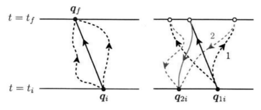
The following describes the framework proposed by Galley for transforming Hamilton’s Principle to a time-asymmetric form. Let $\mathbf{q}$ and $\mathbf{\dot{q}}$ designate sets of $N$ generalized coordinates, plus their velocities, where $\mathbf{q}$ and $\mathbf{\dot{q}}$ are the fundamental variables assumed in the definition of the Lagrangian used by Hamilton’s Principle. As illustrated schematically in Figure $\PageIndex{2}$, Galley proposed doubling the number of degrees of freedom for the system considered, that is, let $\mathbf{q\rightarrow }\left( \mathbf{q}_{1}\mathbf{,q}_{2}\right)$ and $\mathbf{\dot{q}\rightarrow }\left( \mathbf{\dot{q}}_{1}\mathbf{,\dot{q}} _{2}\right)$. In addition he defines two identical variational paths $1$ and $2,$ where path $2$ is the time reverse of path$1$. That is, path $1$ starts at the initial time $t_{i}$, and ends at $t_{f}$, whereas path $2$ starts at $t_{f}$ and ends at $t_{i}$. That is, he assumes that $\mathbf{q}$ and $\mathbf{\dot{q}}$ specify the two paths in the space of the doubled degrees of freedom that are identical, and that they intersect at the final time $t_{f}$. The arrows shown on the paths in Figure $\PageIndex{2}$ designate the assumed direction of the time integration along these paths.

For the doubled system of degrees of freedom, the total action for the sum of the two paths is given by the time integral of the doubled variables, $S( \mathbf{q}_{1},\mathbf{q}_{2})$ which can be written as

$$S\left( \mathbf{q}_{1},\mathbf{q}_{2}\right) =\int_{t_{i}}^{t_{f}}L\left( \mathbf{q}_{1},\mathbf{\dot{q}}_{1}\mathbf{,}t\right) dt+\int_{t_{f}}^{t_{i}}L\left( \mathbf{q}_{2},\mathbf{\dot{q}}_{2},t\right) dt=\int_{t_{i}}^{t_{f}}\left[ L\left( \mathbf{q}_{1},\mathbf{\dot{q}}_{1} \mathbf{,}t\right) dt-L\left( \mathbf{q}_{2},\mathbf{\dot{q}}_{2}\mathbf{,} t\right) \right] dt\label{9.28}$$

The above relation assumes that the doubled variables $\left( \mathbf{q}_{1}, \mathbf{\dot{q}}_{1}\right)$ and $\left( \mathbf{q}_{2},\mathbf{\dot{q}} _{2}\right)$ are decoupled from each other. More generally one can assume that the two sets of variables are coupled by some arbitrary function $K\left( \mathbf{q}_{1},\mathbf{\dot{q}}_{1},\mathbf{q}_{2},\mathbf{\dot{q}} _{2},t\right)$. Then the action can be written as

$$S\left( \mathbf{q}_{1},\mathbf{q}_{2}\right) =\int_{t_{i}}^{t_{f}}\left[ L\left( \mathbf{q}_{1},\mathbf{\dot{q}}_{1}\mathbf{,t}\right) dt-L\left( \mathbf{q}_{2},\mathbf{\dot{q}}_{2}\mathbf{,t}\right) +K\left( \mathbf{q} _{1},\mathbf{\dot{q}}_{1},\mathbf{q}_{2},\mathbf{\dot{q}}_{2},t\right) \right] dt\label{9.29}$$

The effective Lagrangian for this doubled system then can be defined as

$$\Lambda \left( \mathbf{q}_{1},\mathbf{q}_{2},\mathbf{\dot{q}}_{1},\mathbf{ \dot{q}}_{2},t\right) \equiv \left[ L\left( \mathbf{q}_{1},\mathbf{\dot{q}} _{1}\mathbf{,}t\right) dt-L\left( \mathbf{q}_{2},\mathbf{\dot{q}}_{2}\mathbf{ ,}t\right) +K\left( \mathbf{q}_{1},\mathbf{\dot{q}}_{1},\mathbf{q}_{2}, \mathbf{\dot{q}}_{2},t\right) \right]\label{9.30}$$

and the action can be written as $$S\left( \mathbf{q}_{1},\mathbf{q}_{2}\right) =\int_{t_{i}}^{t_{f}}\Lambda \left( \mathbf{q}_{1},\mathbf{\dot{q}}_{1},\mathbf{q}_{2},\mathbf{\dot{q}} _{2},t\right) dt\label{9.31}$$

The coupling term $K\left( \mathbf{q}_{1},\mathbf{\dot{q}}_{1},\mathbf{q} _{2},\mathbf{\dot{q}}_{2},t\right)$ for the doubled system of degrees of freedom must satisfy the following two properties.

(a) If it can be expressed as the difference of two scalar potentials, $\Delta U\left( \mathbf{q}_{1},\mathbf{q}_{2}\right) =U\left( \mathbf{q} _{1}\right) -U\left( \mathbf{q}_{2}\right)$, then it can be absorbed into the potential term for each of the doubled variables in the Lagrangian. This implies that $K=0,$ and there is no reason to double the number of degrees of freedom because the system is conservative. Thus $K$ describes generalized forces that are not derivable from potential energy, that is, conservative.

(b) A second property of the coupling term $K\left( \mathbf{q}_{1},\mathbf{ \dot{q}}_{1},\mathbf{q}_{2},\mathbf{\dot{q}}_{2},t\right)$ is that it must be antisymmetric under interchange of the arbitrary labels $1\leftrightarrow 2$. That is,

$$K\left( \mathbf{q}_{2},\mathbf{\dot{q}}_{2},\mathbf{q}_{1},\mathbf{\dot{q}} _{1},t\right) =-K\left( \mathbf{q}_{1},\mathbf{\dot{q}}_{1},\mathbf{q}_{2}, \mathbf{\dot{q}}_{2},t\right)\label{9.32}$$

Therefore the antisymmetric function $K\left( \mathbf{q}_{1},\mathbf{\dot{q}} _{1},\mathbf{q}_{2},\mathbf{\dot{q}}_{2},t\right)$ vanishes when $\mathbf{q} _{2}=\mathbf{q}_{1}$.

The variational condition requires that the action $S\left( \mathbf{q}_{1}, \mathbf{q}_{2}\right)$ has a well defined stationary point for the doubled system. This is achieved by parametrizing both coordinate paths as

$$\mathbf{q}_{1,2}(t,\epsilon )=\mathbf{q}_{1,2}(t,0)+\epsilon \eta _{1,2}(t)\label{9.33}$$

where $\mathbf{q}_{1,2}(t,0)$ are the coordinates for which the action is stationary, $\epsilon \ll 1.$ and where $\eta _{1,2}(t)$ are arbitrary functions of time denoting virtual displacements of the paths. The doubled system has two independent paths connecting the two initial boundary conditions at $t_{i}$, and it requires that these paths intersect at $t_{f}$. The variational system for the two intersecting paths requires specifying four conditions, two per path. Two of the four conditions are determined by requiring that at $t_{i}$ the initial boundary conditions satisfies that $\eta _{1,2}(t_{i})=0$. The remaining two conditions are derived by requiring that the variation of the action $S\left( \mathbf{q}_{1},\mathbf{q} _{2}\right)$ satisfies

$$\left[ \frac{dS}{d\epsilon }\right] _{\epsilon =0}=0=\int_{t_{i}}^{t_{f}}dt\left\{ \eta _{1}\left[ \frac{\partial \Lambda }{ \partial q_{1}}-\frac{d\pi _{1}}{dt}\right] _{\epsilon =0}-\eta _{2}\left[ \frac{\partial \Lambda }{\partial q_{2}}-\frac{d\pi _{2}}{dt}\right] _{\epsilon =0}\right\} +\left[ \eta _{1}\pi _{1}-\eta _{2}\pi _{2}\right] _{t=t_{f}}\label{9.34}$$

The canonical momenta $\pi _{1,2}$ conjugate to the doubled coordinates $\mathbf{q}_{1,2}$ are defined using the nonconservative Lagrangian $\Lambda$ to be

$$\pi _{1}^{I}\left( \mathbf{q}_{1,2},\mathbf{\dot{q}}_{1,2}\right) \equiv \frac{\partial \Lambda }{\partial \dot{q}_{1}^{I}(t)}=\frac{\partial L\left( \mathbf{q}_{1},\mathbf{\dot{q}}_{1}\mathbf{,}t\right) }{\partial \dot{q} _{1}^{I}(t)}+\frac{\partial K\left( \mathbf{q}_{1},\mathbf{\dot{q}}_{1}, \mathbf{q}_{2},\mathbf{\dot{q}}_{2},t\right) }{\partial \dot{q}_{1}^{I}(t)}\label{9.35}$$

where the superscript $I$ designates the solution based on the initial conditions. Note that the conjugate momentum $p_{1}^{I}=\frac{\partial L\left( \mathbf{q}_{1},\mathbf{\dot{q}}_{1}\mathbf{,}t\right) }{\partial \dot{q}_{1}^{I}(t)}$ while the $\frac{\partial K\left( \mathbf{q}_{1}, \mathbf{\dot{q}}_{1},\mathbf{q}_{2},\mathbf{\dot{q}}_{2},t\right) }{\partial \dot{q}_{1}^{I}(t)}$ term is part of the total momentum due to the nonconservative interaction. Similarly the momentum for the second path is $$\pi _{2}^{I}\left( \mathbf{q}_{1,2},\mathbf{\dot{q}}_{1,2}\right) \equiv \frac{\partial \Lambda }{\partial \dot{q}_{2}^{I}(t)}=\frac{\partial L\left( \mathbf{q}_{1},\mathbf{\dot{q}}_{1}\mathbf{,}t\right) }{\partial \dot{q} _{2}^{I}(t)}+\frac{\partial K\left( \mathbf{q}_{1},\mathbf{\dot{q}}_{1}, \mathbf{q}_{2},\mathbf{\dot{q}}_{2},t\right) }{\partial \dot{q}_{2}^{I}(t)}\label{9.36}$$

The last term in Equation $\ref{9.34}$, that is, the term $\left[ \eta _{1}\pi _{1}-\eta _{2}\pi _{2}\right] _{t=t_{f}}$ results from integration by parts, which will vanish if

$$\eta _{1}^{I}(t_{f})\pi _{1}^{I}(t_{f})=\eta _{2}^{I}(t_{f})\pi _{2}^{I}(t_{f})\label{9.37}$$

The equality condition at the intersection of the two paths at $t_{f}$ requires that

$$\eta _{1}^{I}(t_{f})=\eta _{2}^{I}(t_{f})\label{9.38}$$

Therefore equations $\ref{9.37}$ and $\ref{9.38}$ imply that

$$\pi _{1}^{I}(t_{f})=\pi _{2}^{I}(t_{f})\label{9.39}$$

Therefore equations $\ref{9.38}$ and $\ref{9.39}$ constitute the equality condition that must be satisfied when the two paths intersect at $t_{f}$. The equality condition ensures that the boundary term for integration by parts in Equation $\ref{9.34}$ will vanish for arbitrary variations provided that the two unspecified paths agree at the final time $t_{f}$. Similarly the conjugate momenta $\pi _{1}^{I}(t_{f}),\pi _{2}^{I}(t_{f})$ must agree, but otherwise are unspecified. As a consequence, the equality condition ensures that the variational principle is consistent with the final state at $t_{f}$ not being specified. That is, the equations of motion are only specified by the initial boundary conditions of the time-asymmetric action for the doubled system.

More physics insight is provided by using a more convenient parametrization of the coordinates in terms of their average and difference. That is, let

$$q_{+}^{I}\equiv \frac{q_{1}^{I}+q_{2}^{I}}{2}\hspace{0.85in}q_{-}^{I}\equiv q_{1}^{I}-q_{2}^{I}\label{9.40}$$

Then the physical limit is

$$q_{+}^{I}\rightarrow q^{I}\hspace{0.85in}q_{-}^{I}\rightarrow 0\label{9.41}$$

That is, the average history is the relevant physical history, while the difference coordinate simply vanishes. For these coordinates, the nonconservative Lagrangian is $\Lambda \left( \mathbf{q}_{+},\mathbf{q}_{-}, \mathbf{\dot{q}}_{+},\mathbf{\dot{q}}_{-},t\right)$ and the equality conditions reduce to

$$\begin{align} \pi _{-}(t_{f}) &=&0 \label{9.42}\\ \eta _{-}(t_{f}) &=&0 \label{9.43} \end{align}$$

which implies that the physically relevant average $\left( +\right)$ quantities are not specified at the final time $t_{f}$ in order to have a well-defined variational principle.

The canonical momenta are given by

$$\begin{align} \label{9.44}\pi _{+}^{I} &=&\frac{\pi _{1}^{I}+\pi _{2}^{I}}{2}=\frac{\partial \Lambda }{ \partial \dot{q}_{-}^{I}} \\ \pi _{-}^{I} &=&\pi _{1}^{I}-\pi _{2}^{I}=\frac{\partial \Lambda }{\partial \dot{q}_{+}^{I}}\label{9.45} \end{align}$$

The equations of motion can be written as.

$$\frac{d}{dt}\frac{\partial \Lambda }{\partial \dot{q}_{\pm }^{I}}=\frac{ \partial \Lambda }{\partial q_{\pm }^{I}}\label{9.46}$$

Equation $\ref{9.46}$ is identically zero for the $+$ subscript, while, in the physical limit (PL), the negative subscript gives that

$$\left[ \frac{d}{dt}\frac{\partial \Lambda }{\partial \dot{q}_{-}^{I}}-\frac{ \partial \Lambda }{\partial q_{-}^{I}}\right] _{PL}=0\label{9.47}$$

Substituting for the Lagrangian $\Lambda$ gives that

$$\frac{d}{dt}\frac{\partial L}{\partial \dot{q}_{-}^{I}}-\frac{\partial L}{ \partial q_{-}^{I}}=\left[ \frac{\partial K}{\partial q_{-}^{I}}-\frac{d}{dt} \frac{\partial K}{\partial \dot{q}_{-}^{I}}\right] _{PL}\equiv Q^{I}\left( \mathbf{q}_{1},\mathbf{\dot{q}}_{1}\mathbf{,}t\right)\label{9.48}$$

where $Q^{I}$ is a generalized nonconservative force derived from $K$.

Note that Equation $\ref{9.46}$ can be derived equally well by taking the direct functional derivative with respect to $q_{-}^{I}(t)$, that is, $$0=\left[ \frac{\delta S}{\delta q_{-}^{I}(t)}\right] _{PL}\label{9.49}$$

The above time-asymmetric formalism applies Hamilton’s action principle to systems that involve initial boundary conditions while the second path corresponds to the final boundary conditions. This framework, proposed recently by Galley, provides a remarkable advance for the handling of nonconservative action in Lagrangian and Hamiltonian mechanics.² This formalism directly incorporates the variational principle for initial boundary conditions and causal dynamics that are usually required for applications of Lagrangian and Hamiltonian mechanics. Currently, there is limited exploitation of this new formalism because there has been insufficient time for it to become well known, for full recognition of its importance, and for the development and publication of applications. Chapter $10$ discusses an application of this formalism to nonconservative systems in classical mechanics.

---

²This topic goes beyond the planned scope of this book. It is recommended that the reader refer to the work of Galley, Tsang, and Stein[Gal13, Gal14] for further discussion plus examples of applying this formalism to nonconservative systems in classical mechanics, electromagnetic radiation, RLC circuits, fluid dynamics, and field theory.