11.7: General Features of the Orbit Solutions
- Page ID
- 14111

\( \newcommand{\vecs}[1]{\overset { \scriptstyle \rightharpoonup} {\mathbf{#1}} } \)
\( \newcommand{\vecd}[1]{\overset{-\!-\!\rightharpoonup}{\vphantom{a}\smash {#1}}} \)
\( \newcommand{\id}{\mathrm{id}}\) \( \newcommand{\Span}{\mathrm{span}}\)
( \newcommand{\kernel}{\mathrm{null}\,}\) \( \newcommand{\range}{\mathrm{range}\,}\)
\( \newcommand{\RealPart}{\mathrm{Re}}\) \( \newcommand{\ImaginaryPart}{\mathrm{Im}}\)
\( \newcommand{\Argument}{\mathrm{Arg}}\) \( \newcommand{\norm}[1]{\| #1 \|}\)
\( \newcommand{\inner}[2]{\langle #1, #2 \rangle}\)
\( \newcommand{\Span}{\mathrm{span}}\)
\( \newcommand{\id}{\mathrm{id}}\)
\( \newcommand{\Span}{\mathrm{span}}\)
\( \newcommand{\kernel}{\mathrm{null}\,}\)
\( \newcommand{\range}{\mathrm{range}\,}\)
\( \newcommand{\RealPart}{\mathrm{Re}}\)
\( \newcommand{\ImaginaryPart}{\mathrm{Im}}\)
\( \newcommand{\Argument}{\mathrm{Arg}}\)
\( \newcommand{\norm}[1]{\| #1 \|}\)
\( \newcommand{\inner}[2]{\langle #1, #2 \rangle}\)
\( \newcommand{\Span}{\mathrm{span}}\) \( \newcommand{\AA}{\unicode[.8,0]{x212B}}\)
\( \newcommand{\vectorA}[1]{\vec{#1}} % arrow\)
\( \newcommand{\vectorAt}[1]{\vec{\text{#1}}} % arrow\)
\( \newcommand{\vectorB}[1]{\overset { \scriptstyle \rightharpoonup} {\mathbf{#1}} } \)
\( \newcommand{\vectorC}[1]{\textbf{#1}} \)
\( \newcommand{\vectorD}[1]{\overrightarrow{#1}} \)
\( \newcommand{\vectorDt}[1]{\overrightarrow{\text{#1}}} \)
\( \newcommand{\vectE}[1]{\overset{-\!-\!\rightharpoonup}{\vphantom{a}\smash{\mathbf {#1}}}} \)
\( \newcommand{\vecs}[1]{\overset { \scriptstyle \rightharpoonup} {\mathbf{#1}} } \)
\( \newcommand{\vecd}[1]{\overset{-\!-\!\rightharpoonup}{\vphantom{a}\smash {#1}}} \)
\(\newcommand{\avec}{\mathbf a}\) \(\newcommand{\bvec}{\mathbf b}\) \(\newcommand{\cvec}{\mathbf c}\) \(\newcommand{\dvec}{\mathbf d}\) \(\newcommand{\dtil}{\widetilde{\mathbf d}}\) \(\newcommand{\evec}{\mathbf e}\) \(\newcommand{\fvec}{\mathbf f}\) \(\newcommand{\nvec}{\mathbf n}\) \(\newcommand{\pvec}{\mathbf p}\) \(\newcommand{\qvec}{\mathbf q}\) \(\newcommand{\svec}{\mathbf s}\) \(\newcommand{\tvec}{\mathbf t}\) \(\newcommand{\uvec}{\mathbf u}\) \(\newcommand{\vvec}{\mathbf v}\) \(\newcommand{\wvec}{\mathbf w}\) \(\newcommand{\xvec}{\mathbf x}\) \(\newcommand{\yvec}{\mathbf y}\) \(\newcommand{\zvec}{\mathbf z}\) \(\newcommand{\rvec}{\mathbf r}\) \(\newcommand{\mvec}{\mathbf m}\) \(\newcommand{\zerovec}{\mathbf 0}\) \(\newcommand{\onevec}{\mathbf 1}\) \(\newcommand{\real}{\mathbb R}\) \(\newcommand{\twovec}[2]{\left[\begin{array}{r}#1 \\ #2 \end{array}\right]}\) \(\newcommand{\ctwovec}[2]{\left[\begin{array}{c}#1 \\ #2 \end{array}\right]}\) \(\newcommand{\threevec}[3]{\left[\begin{array}{r}#1 \\ #2 \\ #3 \end{array}\right]}\) \(\newcommand{\cthreevec}[3]{\left[\begin{array}{c}#1 \\ #2 \\ #3 \end{array}\right]}\) \(\newcommand{\fourvec}[4]{\left[\begin{array}{r}#1 \\ #2 \\ #3 \\ #4 \end{array}\right]}\) \(\newcommand{\cfourvec}[4]{\left[\begin{array}{c}#1 \\ #2 \\ #3 \\ #4 \end{array}\right]}\) \(\newcommand{\fivevec}[5]{\left[\begin{array}{r}#1 \\ #2 \\ #3 \\ #4 \\ #5 \\ \end{array}\right]}\) \(\newcommand{\cfivevec}[5]{\left[\begin{array}{c}#1 \\ #2 \\ #3 \\ #4 \\ #5 \\ \end{array}\right]}\) \(\newcommand{\mattwo}[4]{\left[\begin{array}{rr}#1 \amp #2 \\ #3 \amp #4 \\ \end{array}\right]}\) \(\newcommand{\laspan}[1]{\text{Span}\{#1\}}\) \(\newcommand{\bcal}{\cal B}\) \(\newcommand{\ccal}{\cal C}\) \(\newcommand{\scal}{\cal S}\) \(\newcommand{\wcal}{\cal W}\) \(\newcommand{\ecal}{\cal E}\) \(\newcommand{\coords}[2]{\left\{#1\right\}_{#2}}\) \(\newcommand{\gray}[1]{\color{gray}{#1}}\) \(\newcommand{\lgray}[1]{\color{lightgray}{#1}}\) \(\newcommand{\rank}{\operatorname{rank}}\) \(\newcommand{\row}{\text{Row}}\) \(\newcommand{\col}{\text{Col}}\) \(\renewcommand{\row}{\text{Row}}\) \(\newcommand{\nul}{\text{Nul}}\) \(\newcommand{\var}{\text{Var}}\) \(\newcommand{\corr}{\text{corr}}\) \(\newcommand{\len}[1]{\left|#1\right|}\) \(\newcommand{\bbar}{\overline{\bvec}}\) \(\newcommand{\bhat}{\widehat{\bvec}}\) \(\newcommand{\bperp}{\bvec^\perp}\) \(\newcommand{\xhat}{\widehat{\xvec}}\) \(\newcommand{\vhat}{\widehat{\vvec}}\) \(\newcommand{\uhat}{\widehat{\uvec}}\) \(\newcommand{\what}{\widehat{\wvec}}\) \(\newcommand{\Sighat}{\widehat{\Sigma}}\) \(\newcommand{\lt}{<}\) \(\newcommand{\gt}{>}\) \(\newcommand{\amp}{&}\) \(\definecolor{fillinmathshade}{gray}{0.9}\)It is useful to look at the general features of the solutions of the equations of motion given by the equivalent one-body representation of the two-body motion. These orbits depend on the net center of mass energy \(E_{cm}.\) There are five possible situations depending on the center-of-mass total energy \(E_{cm}\).
- \(\mathbf{E}_{cm}\mathbf{>0}:\) The trajectory is hyperbolic and has a minimum distance, but no maximum. The distance of closest approach is given when \(\dot{r}=0.\) At the turning point \(E_{cm}=U+\) \(\frac{l^{2}}{2\mu r^{2}}\)
- \(\mathbf{E}_{cm}\mathbf{=0}:\) It can be shown that the orbit for this case is parabolic.
- \(\mathbf{0>E}_{cm}\mathbf{>U}_{\min }:\) For this case the equivalent orbit has both a maximum and minimum radial distance at which \(\dot{r}=0.\) At the turning points the radial kinetic energy term is zero so \(E_{cm}=U+\) \(\frac{l^{2}}{2\mu r^{2}}.\) For the attractive inverse square law force the path is an ellipse with the focus at the center of attraction (Figure \((11.8.1)\)), which is Kepler’s First Law. During the time that the radius ranges from \(r_{\min }\) to \(r_{\max }\) and back the radius vector turns through an angle \(\Delta \psi\) which is given by
\[\Delta \psi =2\int_{r_{\min }}^{r_{\max }}\frac{\pm ldr}{r^{2}\sqrt{2\mu \left( E_{cm}-U-\frac{l^{2}}{2\mu r^{2}}\right) }}\]
The general path prescribes a rosette shape which is a closed curve only if \(\Delta \psi\) is a rational fraction of \(2\pi\).
- \(\mathbf{E}_{cm}\mathbf{=U}_{\min }:\) In this case \(r\) is a constant implying that the path is circular since \[\dot{r}=\frac{dr}{dt}=\pm \sqrt{\frac{2}{\mu }\left( E_{cm}-U-\frac{l^{2}}{ 2\mu r^{2}}\right) }=0\]
- \(\mathbf{E}_{cm}\mathbf{<U}_{\min }:\) For this case the square root is imaginary and there is no real solution.
In general the orbit is not closed, and such open orbits do not repeat. Bertrand’s Theorem states that the inverse-square central force, and the linear harmonic oscillator, are the only radial dependences of the central force that lead to stable closed orbits.
Example \(\PageIndex{1}\): Orbit equation of motion for a free body
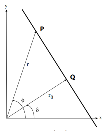
It is illustrative to use the differential orbit equation \((11.5.1)\) to show that a body in free motion travels in a straight line. Assume that a line through the origin \(O\) intersects perpendicular to the instantaneous trajectory at the point \(Q\) which has polar coordinates \((r_{0},\phi )\) relative to the origin. The point \(P,\) with polar coordinates \((r,\phi ),\) lies on a straight line through \(Q\) that is perpendicular to \(OQ\) if, and only if, \(r\cos (\phi -\delta )=r_{0}.\) Since the force is zero then the differential orbit equation simplifies to
\[\frac{d^{2}u(\phi )}{d\phi ^{2}}+u(\phi )=0\notag\]
A solution of this is
\[u(\phi )=\frac{1}{r_{0}}\cos (\phi -\delta )\notag\]
where \(r_{0}\) and \(\delta\) are arbitrary constants. This can be rewritten as
\[r(\phi )=\frac{r_{0}}{\cos (\phi -\delta )} \notag\]
This is the equation of a straight line in polar coordinates as illustrated in the adjacent figure. This shows that a free body moves in a straight line if no forces are acting on the body.