11.8: Inverse-square, two-body, central force

The most important conservative, two-body, central interaction is the attractive inverse-square law force, which is encountered in both gravitational attraction and the Coulomb force. This force \(\mathbf{F(r)}\) can be written in the form

\[\mathbf{F}(r)= \frac{k}{r^{2}}\widehat{\mathbf{r}}\label{11.52}\]

The force constant \(k\) is defined to be negative for an attractive force and positive for a repulsive force. In S.I. units the force constant \(k=-Gm_{1}m_{2}\) for the gravitational force and \(k=+\frac{q_{1}q_{2}}{4\pi \epsilon _{0}}\) for the Coulomb force. Note that this sign convention is the opposite of what is used in many books which use a negative sign in Equation \ref{11.52} and assume \(k\) to be positive for an attractive force and negative for a repulsive force.

The conservative, inverse-square, two-body, central force is unique in that the underlying symmetries lead to four conservation laws, all of which are of pivotal importance in nature.

1. Conservation of angular momentum: Like all conservative central forces, the inverse-square central two-body force conserves angular momentum as proven in chapter \(11.3\).
2. Conservation of energy: This conservative central force can be represented in terms of a scalar potential energy \(U(r)\) as given by equation \((11.1.2)\), where for this central force

   \[U(r)=\frac{k}{r}\label{11.53}\]

   Moreover, equation \((11.6.3)\) showed that the center-of-mass Hamiltonian is conserved, that is, \(H_{cm}=E_{cm}\)

3. Gauss’ Law: For a conservative, inverse-square, two-body, central force, the flux of the force field out of any closed surface is proportional to the algebraic sum of the sources and sinks of this field that are located inside the closed surface. The net flux is independent of the distribution of the sources and sinks inside the closed surface, as well as the size and shape of the closed surface. Chapter \(2.14.5\) proved this for the gravitational force field.
4. Closed orbits: Two bodies interacting via the conservative, inverse-square, two-body, central force follow closed (degenerate) orbits as stated by Bertrand’s Theorem. The first consequence of this symmetry is that Kepler’s laws of planetary motion have stable, single-valued orbits. The second consequence of this symmetry is the conservation of the eccentricity vector defined in Equation \ref{11.86}.

Observables that depend on Gauss’s Law, or on closed planetary orbits, are extremely sensitive to addition of even a miniscule incremental exponent \(\xi\) to the radial dependence \(r^{-\left( 2\pm \xi \right) }\) of the force. The statement that the inverse-square, two-body, central force leads to closed orbits can be proven by inserting Equation \ref{11.52} into the orbit differential equation,

\[\frac{d^{2}u}{d\psi ^{2}}+u=-\frac{\mu }{l^{2}}\frac{1}{u^{2}}ku^{2}=-\frac{ \mu k}{l^{2}}\]

Using the transformation

\[y\equiv u+\frac{\mu k}{l^{2}}\]

the orbit equation becomes

\[\frac{d^{2}y}{d\psi ^{2}}+y=0\]

A solution of this equation is

\[y=B\cos \left( \psi -\psi _{0}\right)\]

Therefore

\[u=\frac{1}{r}=-\frac{\mu k}{l^{2}}\left[ 1+\epsilon \cos \left( \psi -\psi _{0}\right) \right]\label{11.58}\]

This is the equation of a conic section. For an attractive, inverse-square, central force, Equation \ref{11.58} is the equation for an ellipse with the origin of \(r\) at one of the foci of the ellipse that has eccentricity \(\epsilon ,\) defined as \[\epsilon \equiv B\frac{l^{2}}{\mu k}\label{11.59}\]

Equation \ref{11.58} is the polar equation of a conic section. Equation \ref{11.58} also can be derived with the origin at a focus by inserting the inverse square law potential into equation \((11.6.10)\) which gives

\[\psi =\int \frac{\pm du}{\sqrt{\frac{2\mu E_{cm}}{l^{2}}+\frac{2\mu k}{l^{2}} u-u^{2}}}+\text{ constant}\label{11.60}\]

The solution of this gives

\[u=\frac{1}{r}=-\frac{\mu k}{l^{2}}\left[ 1+\sqrt{1+\frac{2E_{cm}l^{2}}{\mu k^{2}}}\cos \left( \psi -\psi _{0}\right) \right]\label{11.61}\]

Equations \ref{11.58} and \ref{11.61} are identical if the eccentricity \(\epsilon\) equals

\[\epsilon =\sqrt{1+\frac{2E_{cm}l^{2}}{\mu k^{2}}}\label{11.62}\]

The value of \(\psi _{0}\) merely determines the orientation of the major axis of the equivalent orbit. Without loss of generality, it is possible to assume that the angle \(\psi\) is measured with respect to the major axis of the orbit, that is \(\psi _{0}=0\). Then the equation can be written as

\[u=\frac{1}{r}=-\frac{\mu k}{l^{2}}\left[ 1+\epsilon \cos \left( \psi \right) \right] =-\frac{\mu k}{l^{2}}\left[ 1+\sqrt{1+\frac{2E_{cm}l^{2}}{\mu k^{2}}} \cos \left( \psi \right) \right]\label{11.63}\]

This is the equation of a conic section where \(\epsilon\) is the eccentricity of the conic section. The conic section is a hyperbola if \(\epsilon >1\), parabola if \(\epsilon =1,\) ellipse if \(\epsilon <1,\) and a circle if \(\epsilon =0.\) All the equivalent one-body orbits for an attractive force have the origin of the force at a focus of the conic section. The orbits depend on whether the force is attractive or repulsive, on the conserved angular momentum \(l,\) and on the center-of-mass energy \(E_{cm}\).

Bound orbits

Closed bound orbits occur only if the following requirements are satisfied.

1. The force must be attractive, \((k<0)\) then Equation \ref{11.63} ensures that \(r\) is positive.
2. For a closed elliptical orbit. the eccentricity \(\epsilon <1\) of the equivalent one-body representation of the orbit implies that the total center-of-mass energy \(E_{cm}<0\), that is, the closed orbit is bound.

Bound elliptical orbits have the center-of-force at one interior focus \(F_{1}\) of the elliptical one-body representation of the orbit as shown in Figure \(\PageIndex{1}\).

Figure \(\PageIndex{1}\): Bound elliptical orbit.

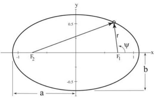
The minimum value of the orbit \(r=r_{\min }\) occurs when \(\psi =0,\) where

\[r_{\min }=- \frac{l^{2}}{\mu k\left[ 1+\epsilon \right] }\label{11.64}\]

This minimum distance is called the periapsis¹.

The maximum distance, \(r=r_{\max },\) which is called the apoapsis, occurs when \(\psi =180^{o}\)

\[r_{\max }=- \frac{l^{2}}{\mu k\left[ 1-\epsilon \right] }\label{11.65}\]

Remember that since \(k<0\) for bound orbits, the negative signs in equations \ref{11.64} and \ref{11.65} lead to \(r>0\). The most bound orbit is a circle having \(\epsilon =0\) which implies that \(E_{cm}=-\frac{\mu k^{2}}{l^{2}}\).

The shape of the elliptical orbit also can be described with respect to the center of the elliptical equivalent orbit by deriving the lengths of the semi-major axis \(a\) and the semi-minor axis \(b\) shown in Figure \(\PageIndex{1}\). \[\begin{align} a &=&\frac{1}{2}\left( r_{\min }+r_{\max }\right) =\frac{1}{2}\left( \frac{ l^{2}}{\mu k\left[ 1+\epsilon \right] }+\frac{l^{2}}{\mu k\left[ 1-\epsilon \right] }\right) =\frac{l^{2}}{\mu k\left[ 1-\epsilon ^{2}\right] }\label{11.66} \\ b &=&a\sqrt{1-\epsilon ^{2}}=\frac{l^{2}}{\mu k\sqrt{[1-\epsilon ^{2}]}}\label{11.67} \end{align}\]

Remember that the predicted bound elliptical orbit corresponds to the equivalent one-body representation for the two-body motion as illustrated in Figure \((11.2.2)\). This can be transformed to the individual spatial trajectories of the each of the two bodies in an inertial frame.

Kepler’s laws for bound planetary motion

Kepler’s three laws of motion apply to the motion of two bodies in a bound orbit due to the attractive gravitational force for which \(k=-Gm_{1}m_{2}\).

1. Each planet moves in an elliptical orbit with the sun at one focus
2. The radius vector, drawn from the sun to a planet, describes equal areas in equal times
3. The square of the period of revolution about the sun is proportional to the cube of the major axis of the orbit.

Two bodies interacting via the gravitational force, which is a conservative, inverse-square, two-body central force, is best handled using the equivalent orbit representation. The first and second laws were proved in chapters \(11.8\) and \(11.3\). That is, the second law is equivalent to the statement that the angular momentum is conserved. The third law can be derived using the fact that the area of an ellipse is

\[A=\pi ab=\pi a^{2} \sqrt{1-\epsilon ^{2}}=\frac{\pi l}{\sqrt{-\mu k}}a^{\frac{3}{2}}\]

Equations \((11.3.7)\) and \((11.3.8)\) give that the rate of change of area swept out by the radius vector is

\[\frac{dA}{dt}=\frac{1}{2}r^{2}\dot{\psi}=\frac{l}{2\mu }\]

Therefore the period for one revolution \(\tau\) is given by the time to sweep out one complete ellipse

\[\tau =\frac{A}{\left( \frac{dA}{dt}\right) }=2\pi \left( \frac{\mu }{-k} \right) ^{\frac{1}{2}}a^{\frac{3}{2}}\]

This leads to Kepler’s \(3^{rd}\) law \[\tau ^{2}=4\pi ^{2}\frac{\mu }{-k}a^{3}\label{11.71}\]

Bound orbits occur only for attractive forces for which the force constant \(k\) is negative, and thus cancel the negative sign in Equation \ref{11.71}. For example, for the gravitational force \(k=-Gm_{1}m_{2}\).

Note that the reduced mass \(\mu =\frac{m_{1}m_{2}}{m_{1}+m_{2}}\) occurs in Kepler’s \(3^{rd}\) law. That is, Kepler’s third law can be written in terms of the actual masses of the bodies to be

\[\tau ^{2}=\frac{4\pi ^{2}}{G\left( m_{1}+m_{2}\right) }a^{3}\label{11.72}\]

In relating the relative periods of the different planets Kepler made the approximation that the mass of the planet \(m_{1}\) is negligible relative to the mass of the sun \(m_{2}.\)

The eccentricity of the major planets ranges from \(\epsilon =0.2056\) for Mercury, to \(\epsilon =0.0068\) for Venus. The Earth has an eccentricity of \(\epsilon =0.0167\) with \(r_{\min }=91\cdot 10^{6\text{ }}\)miles and \(r_{\max }=95\cdot 10^{6}\) miles. On the other hand, \(\epsilon =0.967\) for Halley’s comet, that is, the radius vector ranges from \(0.6\) to \(18\) times the radius of the orbit of the Earth.

The orbit energy can be derived by substituting the eccentricity, given by Equation \ref{11.62}, into the semi-major axis length \(a,\) given by Equation \ref{11.66}, which leads to the center-of-mass energy of

\[E_{cm}=-\frac{k}{2a}\]

However, the Hamiltonian, given by equation \((11.6.3)\), implies that \(E_{cm}\) is

\[E_{cm}=\frac{1}{2}\mu v^{2}+\left( -\frac{k}{r}\right) =-\frac{k}{2a}\]

For the simple case of a circular orbit, \(a=r\) then the velocity \(v\) equals \[v=\sqrt{\frac{k}{\mu r}}\]

For a circular orbit, the drag on a satellite lowers the total energy resulting in a decrease in the radius of the orbit and a concomitant increase in velocity. That is, when the orbit radius is decreased, part of the gain in potential energy accounts for the work done against the drag, and the remaining part goes towards increase of the kinetic energy. Also note that, as predicted by the Virial Theorem, the kinetic energy always is half the potential energy for the inverse square law force.

Unbound orbits

Attractive inverse-square central forces lead to hyperbolic orbits for \(\epsilon >1\) for which \(E_{cm}>0\), that is, the orbit is unbound. In addition, the orbits always are unbound for a repulsive force since \(U=\frac{ k}{r}\) is positive as is the kinetic energy \(T_{cm}\), thus \(E_{cm}=T_{cm}+U_{cm}>0\). The radial orbit equation for either an attractive or a repulsive force is

\[r=- \frac{l^{2}}{\mu k\left[ 1+\epsilon \cos \psi \right] }\]

For a repulsive force \(k\) is positive and \(l^{2}\) always is positive. Therefore to ensure that \(r\) remain positive the bracket term must be negative. That is

\[\left[ 1+\epsilon \cos \psi \right] <0\hspace{1in}k>0\]

For an attractive force \(k\) is negative and since \(l^{2}\) is positive then the bracket term must be positive to ensure that \(r\) is positive. That is, \[\left[ 1+\epsilon \cos \psi \right] >0\hspace{1in}k<0\]

Figure \(\PageIndex{2}\): Hyperbolic two-body orbits for a repulsive (left) and attractive (right) inverse-square, central two-body forces. Both orbits have the angular momentum vector pointing upwards out of the plane of the orbit

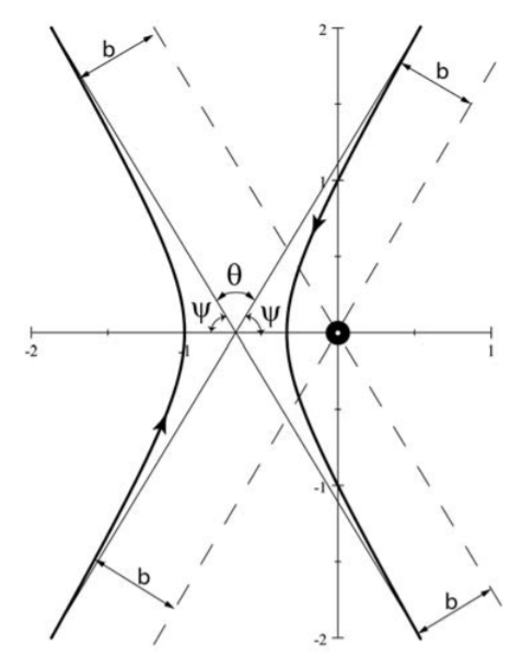
Figure \(\PageIndex{2}\) shows both branches of the hyperbola for a given angle \(\psi\) for the equivalent two-body orbits where the center of force is at the origin. For an attractive force, \(k<0,\) the center of force is at the interior focus of the hyperbola, whereas for a repulsive force the center of force is at the exterior focus. For a given value of \(\left\vert \psi \right\vert\) the asymptotes of the orbits both are displaced by the same impact parameter \(b\) from parallel lines passing through the center of force. The scattering angle, between the outgoing direction of the scattered body and the incident direction, is designated to be \(\theta ,\) which is related to the angle \(\psi\) by \(\theta =180^{\circ }-2\psi\).

Eccentricity vector

Two-bodies interacting via a conservative two-body central force have two invariant first-order integrals, namely the conservation of energy and the conservation of angular momentum. For the special case of the inverse-square law, there is a third invariant of the motion, which Hamilton called the eccentricity vector², that unambiguously defines the orientation and direction of the major axis of the elliptical orbit. It will be shown that the angular momentum plus the eccentricity vector completely define the plane and orientation of the orbit for a conservative inverse-square law central force.

Newton’s second law for a central force can be written in the form

\[\mathbf{ \dot{p}=}f(r)\mathbf{\hat{r}}\]

Note that the angular moment \(\mathbf{L}=\mathbf{r\times p}\) is conserved for a central force, that is \(\mathbf{\dot{L}}=0\). Therefore the time derivative of the product \(\mathbf{p\times L}\) reduces to

\[\frac{d}{dt}\left( \mathbf{p\times L}\right) \mathbf{=\dot{p}\times L=}f(r) \mathbf{\hat{r}\times }\left( \mathbf{r\times }\mu \mathbf{\dot{r}}\right) =f(r)\frac{\mu }{r}\left[ \mathbf{r}\left( \mathbf{r\cdot \dot{r}}\right) -r^{2}\mathbf{\dot{r}}\right]\label{11.80}\]

This can be simplified using the fact that

\[\mathbf{r\cdot \dot{r}=}\frac{1}{2}\frac{d}{dt}\left( \mathbf{r\cdot r} \right) =r\dot{r}\]

thus

\[f(r)\frac{\mu }{r}\left[ \mathbf{r}\left( \mathbf{r\cdot \dot{r}}\right) -r^{2}\mathbf{\dot{r}}\right] =-\mu f(r)r^{2}\left[ \frac{\mathbf{\dot{r}}}{r }-\frac{\mathbf{r}\dot{r}}{r^{2}}\right] =-\mu f(r)r^{2}\frac{d}{dt}\left( \frac{\mathbf{r}}{r}\right)\]

This allows Equation \ref{11.80} to be reduced to

\[\frac{d}{dt}\left( \mathbf{p\times L}\right) \mathbf{=}-\mu f(r)r^{2}\frac{d }{dt}\left( \frac{\mathbf{r}}{r}\right)\label{11.83}\]

Assume the special case of the inverse-square law, Equation \ref{11.52}, then the central force Equation \ref{11.83} reduces to

\[\frac{d}{dt}\left( \mathbf{p\times L}\right) \mathbf{=-}\frac{d}{dt}\left( \mu k\mathbf{\hat{r}}\right)\label{11.84}\]

or

\[\frac{d}{dt}\left[ \left( \mathbf{p\times L}\right) \mathbf{+}\left( \mu k \mathbf{\hat{r}}\right) \right] =0\label{11.85}\]

Define the eccentricity vector \(\mathbf{A}\) as

\[\mathbf{A\equiv }\left( \mathbf{p\times L}\right) \mathbf{+}\left( \mu k \mathbf{\hat{r}}\right)\label{11.86}\]

then Equation \ref{11.85} corresponds to

\[\frac{d\mathbf{A}}{dt}=0\label{11.87}\]

This is a statement that the eccentricity vector \(A\) is a constant of motion for an inverse-square, central force.

The definition of the eccentricity vector \(\mathbf{A}\) and angular momentum vector \(\mathbf{L}\) implies a zero scalar product,

\[\mathbf{A\cdot L=}0\label{11.88}\]

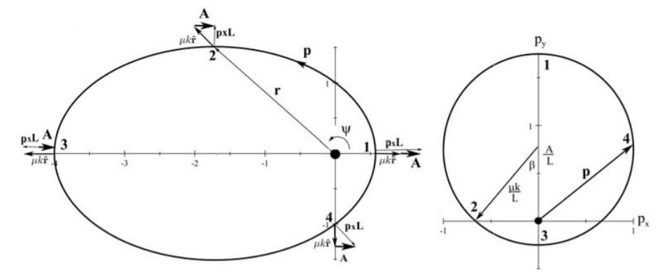
Thus the eccentricity vector \(\mathbf{A}\) and angular momentum \(\mathbf{L}\) are mutually perpendicular, that is, \(\mathbf{A}\) is in the plane of the orbit while \(\mathbf{L}\) is perpendicular to the plane of the orbit. The eccentricity vector \(\mathbf{A}\), always points along the major axis of the ellipse from the focus to the periapsis as illustrated on the left side in Figure \(\PageIndex{3}\). As a consequence, the two orthogonal vectors \(\mathbf{ A}\) and \(\mathbf{L}\) completely define the plane of the orbit, plus the orientation of the major axis of the Kepler orbit, in this plane. The three vectors \(\mathbf{A}\), \(\mathbf{p\times L}\), and \(\left( \mu k\mathbf{\hat{r}} \right)\) obey the triangle rule as illustrated in the left side of Figure \(\PageIndex{3}\).

Figure \(\PageIndex{3}\): The elliptical trajectory and eccentricity vector \(\mathbf{A}\) for two bodies interacting via the inversesquare, central force for eccentricity \(\epsilon = 0.75\). The left plot shows the elliptical spatial trajectory where the semi-major axis is assumed to be on the \(x\)-axis and the angular momentum \(\mathbf{L} =l \hat{\mathbf{z}}\), is out of the page. The force centre is at one foci of the ellipse. The vector coupling relation \(\mathbf{A} \equiv (\mathbf{p} \times \mathbf{L}) + (\mu k \hat{\mathbf{r}})\) is illustrated at four points on the spatial trajectory. The right plot is a hodograph of the linear momentum \(\mathbf{p}\) for this trajectory. The periapsis is denoted by the number \(\mathbf{1}\) and the apoapsis is marked as \(\mathbf{3}\) on both plots. Note that the eccentricity vector \(\mathbf{A}\) is a constant that points parallel to the major axis towards the perapsis.

Hamilton noted the direct connection between the eccentricity vector \(\mathbf{A}\) and the eccentricity \(\epsilon\) of the conic section orbit. This can be shown by considering the scalar product

\[\mathbf{A\cdot r=}Ar\cos \psi =\mathbf{r\cdot }\left( \mathbf{p\times L} \right) +\mu kr\label{11.89}\]

Note that the triple scalar product can be permuted to give

\[\mathbf{r\cdot }\left( \mathbf{p\times L}\right) =\left( \mathbf{r}\times \mathbf{p}\right) \mathbf{\cdot L=L\cdot L=}l^{2}\label{11.90}\]

Inserting Equation \ref{11.90} into \ref{11.89} gives \[\frac{1}{r}=-\frac{\mu k}{l^{2}}\left( 1-\frac{A}{\mu k}\cos \psi \right)\label{11.91}\]

Note that equations \ref{11.63} and \ref{11.91} are identical if \(\psi _{0}=0\). This implies that the eccentricity \(\epsilon\) and \(A\) are related by

\[\epsilon =-\frac{A}{\mu k}\label{11.92}\]

where \(k\) is defined to be negative for an attractive force. The relation between the eccentricity and total center-of-mass energy can be used to rewrite Equation \ref{11.62} in the form \[A^{2}=\mu ^{2}k^{2}+2\mu E_{cm}l^{2}\label{11.93}\]

The combination of the eccentricity vector \(\mathbf{A}\) and the angular momentum vector \(\mathbf{L}\) completely specifies the orbit for an inverse square-law central force. The trajectory is in the plane perpendicular to the angular momentum vector \(\mathbf{L}\), while the eccentricity, plus the orientation of the orbit, both are defined by the eccentricity vector \(\mathbf{A}\). The eccentricity vector and angular momentum vector each have three independent coordinates, that is, these two vector invariants provide six constraints, while the scalar invariant energy \(E,\) adds one additional constraint. The exact location of the particle moving along the trajectory is not defined and thus there are only five independent coordinates governed by the above seven constraints. Thus the eccentricity vector, angular momentum, and center-of-mass energy are related by the two equations \ref{11.88} and \ref{11.93}.

Noether’s theorem states that each conservation law is a manifestation of an underlying symmetry. Identification of the underlying symmetry responsible for the conservation of the eccentricity vector \(\mathbf{A}\) is elucidated using Equation \ref{11.86} to give

\[\left( \mu k\mathbf{\hat{r}}\right) =\mathbf{A-}\left( \mathbf{p\times L} \right)\] Take the scalar product

\[\left( \mu k\mathbf{\hat{r}}\right) \cdot \left( \mu k\mathbf{\hat{r}} \right) =\left( \mu k\right) ^{2}=p^{2}L^{2}+A^{2}-2L\cdot \left( \mathbf{ p\times L}\right)\]

Choose the angular momentum to be along the \(z\)-axis, that is, \(\mathbf{L=}l \mathbf{\hat{z}}\), and, since \(\mathbf{p}\) and \(\mathbf{A}\) are perpendicular to \(\mathbf{L}\), then \(\mathbf{p}\) and \(\mathbf{A}\) are in the \(\mathbf{\hat{x}-\hat{y}}\) plane. Assume that the semimajor axis of the elliptical orbit is along the \(\mathbf{x}\)-axis, then the locus of the momentum vector on a momentum hodograph has the equation

\[p_{x}^{2}+\left( p_{y}-\frac{A}{L}\right) ^{2}=\left( \frac{\mu k}{L}\right) ^{2}\label{11.96}\]

Equation \ref{11.96} implies that the locus of the momentum vector is a circle of radius \(\left\vert \frac{\mu k}{L}\right\vert\) with the center displaced from the origin at coordinates \(\left( 0,\frac{A}{L}\right)\) as shown by the momentum hodograph on the right side of an Figure \(\PageIndex{3}\). The angle \(\beta\) and eccentricity \(\epsilon\) are related by,

\[\cos \beta =-\frac{A/L}{\mu k/L}=-\frac{A}{\mu k}=\epsilon\]

The circular orbit is centered at the origin for \(\epsilon =-\frac{A}{\mu k} =0\), and thus the magnitude \(\left\vert \mathbf{p}\right\vert\) is a constant around the whole trajectory.

The inverse-square, central, two-body, force is unusual in that it leads to stable closed bound orbits because the radial and angular frequencies are degenerate, i.e. \(\omega _{r}=\omega _{\psi }.\) In momentum space, the locus of the linear momentum vector \(\mathbf{p}\) is a perfect circle which is the underlying symmetry responsible for both the fact that the orbits are closed, and the invariance of the eccentricity vector. Mathematically this symmetry for the Kepler problem corresponds to the body moving freely on the boundary of a four-dimensional sphere in space and momentum. The invariance of the eccentricity vector is a manifestation of the special property of the inverse-square, central force under certain rotations in this four-dimensional space; this \(O(4)\) symmetry is an example of a hidden symmetry.

---

¹The greek term apsis refers to the points of greatest or least distance of approach for an orbiting body from one of the foci of the elliptical orbit. The term periapsis or pericenter both are used to designate the closest distance of approach, while apoapsis or apocenter are used to designate the farthest distance of approach. Attaching the terms "perí-" and "apo-" to the general term "-apsis" is preferred over having different names for each object in the solar system. For example, frequently used terms are "-helion" for orbits of the sun, "-gee" for orbits around the earth, and "-cynthion" for orbits around the moon.

²The symmetry underlying the eccentricity vector is less intuitive than the energy or angular momentum invariants leading to it being discovered independently several times during the past three centuries. Jakob Hermann was the first to indentify this invariant for the special case of the inverse-square central force. Bernoulli generalized his proof in 1710. Laplace derived the invariant at the end of the 18th century using analytical mechanics. Hamilton derived the connection between the invariant and the orbit eccentricity. Gibbs derived the invariant using vector analysis. Runge published the Gibb’s derivation in his textbook which was referenced by Lenz in a 1924 paper on the quantal model of the hydrogen atom. Goldstein named this invariant the "Laplace-Runge-Lenz vector", while others have named it the "Runge-Lenz vector" or the "Lenz vector". This book uses Hamilton’s more intuitive name of "eccentricity vector".