11.9: Isotropic, linear, two-body, central force

Closed orbits occur for the two-dimensional linear oscillator when \(\frac{\omega _{x}}{\omega _{y}}\) is a rational fraction as discussed in chapter \(3.3\). Bertrand’s Theorem states that the linear oscillator, and the inverse-square law (Kepler problem), are the only two-body central forces that have single-valued, stable, closed orbits of the coupled radial and angular motion. The invariance of the eccentricity vector was the underlying symmetry leading to single-valued, stable, closed orbits for the Kepler problem. It is interesting to explore the symmetry that leads to stable closed orbits for the harmonic oscillator. For simplicity, this discussion will restrict discussion to the isotropic, harmonic, two-body, central force where \(\omega _{x}=\omega _{y}=\omega\), for which the two-body, central force is linear

\[\mathbf{F}(r)=k\mathbf{r}\label{11.98}\]

where \(k>0\) corresponds to a repulsive force and \(k<0\) to an attractive force. This isotropic harmonic force can be expressed in terms of a spherical potential \(U(r)\) where

\[U(r)=- \frac{1}{2}kr^{2}\label{11.99}\]

Since this is a central two-body force, both the equivalent one-body representation, and the conservation of angular momentum, are equally applicable to the harmonic two-body force. As discussed in section \(11.3\), since the two-body force is central, the motion is confined to a plane, and thus the Lagrangian can be expressed in polar coordinates. In addition, since the force is spherically symmetric, then the angular momentum is conserved. The orbit solutions are conic sections as described in chapter \(11.7\). The shape of the orbit for the harmonic two-body central force can be derived using either polar or cartesian coordinates as illustrated below.

Polar coordinates

The origin of the equivalent orbit for the harmonic force will be found to be at the center of an ellipse, rather than the foci of the ellipse as found for the inverse square law. The shape of the orbit can be defined using a Binet differential orbit equation that employs the transformation

\[u^{\prime }\equiv \frac{1}{r^{2}}\label{11.100}\]

Then

\[\frac{du^{\prime }}{d\psi }=-\frac{2}{r^{3}}\frac{dr}{d\psi }\label{11.101}\]

The chain rule gives that

\[\dot{r}=\frac{dr}{d\psi }\dot{\psi}=-\frac{r^{3}}{2}\dot{\psi}\frac{ du^{\prime }}{d\psi }=-\frac{r}{2}\frac{p_{\psi }}{\mu }\frac{du^{\prime }}{ d\psi }\label{11.102}\]

Substitute this into the Hamiltonian \(H_{cm},\) equation \((11.6.3)\), gives

\[\frac{1}{2}\mu \dot{r}^{2}=\frac{1}{8}\frac{p_{\psi }^{2}}{u^{\prime }\mu } \left( \frac{du^{\prime }}{d\psi }\right) ^{2}=E-\frac{p_{\psi }^{2}}{2\mu } u^{\prime }+\frac{k}{2u^{\prime }}\label{11.103}\]

Rearranging this equation gives

\[\left( \frac{du^{\prime }}{d\psi }\right) ^{2}+4u^{\prime 2}-\frac{8E\mu }{ p_{\psi }^{2}}u^{\prime }=\frac{4k\mu }{p_{\psi }^{2}}\label{11.104}\]

Addition of a constant to both sides of the equation completes the square

\[\left[ \frac{d}{d\psi }\left( u^{\prime }-\frac{E\mu }{p_{\psi }^{2}}\right) \right] ^{2}+4\left( u^{\prime }-\frac{E\mu }{p_{\psi }^{2}}\right) ^{2}=+ \frac{4k\mu }{p_{\psi }^{2}}+4\left( \frac{E\mu }{p_{\psi }^{2}}\right) ^{2}\label{11.105}\]

The right-hand side of Equation \ref{11.105} is a constant. The solution of \ref{11.105} must be a sine or cosine function with polar angle \(\psi =\omega t\). That is

\[\left( u^{\prime }-\frac{E\mu }{p_{\psi }^{2}}\right) =\left[ \left( \frac{ E\mu }{p_{\psi }^{2}}\right) ^{2}+\frac{k\mu }{p_{\psi }^{2}}\right] ^{\frac{ 1}{2}}\cos 2\left( \psi -\psi _{0}\right)\label{11.106}\]

That is,

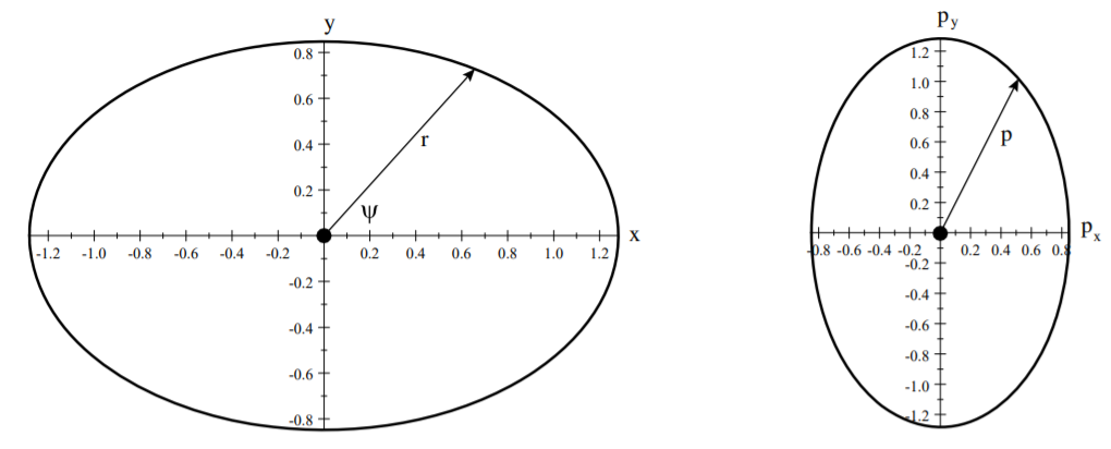
\[u^{\prime }=\frac{1}{r^{2}}=\frac{E\mu }{p_{\psi }^{2}}\left( 1+\left( 1+ \frac{kp_{\psi }^{2}}{E^{2}\mu }\right) ^{\frac{1}{2}}\cos 2(\psi -\psi _{0})\right)\label{11.107}\] Equation \ref{11.107} corresponds to a closed orbit centered at the origin of the elliptical orbit as illustrated in Figure \(\PageIndex{1}\). The eccentricity \(\epsilon\) of this closed orbit is given by

\[\left( 1+\frac{kp_{\psi }^{2}}{E^{2}\mu }\right) ^{\frac{1}{2}}=\frac{ \epsilon ^{2}}{2-\epsilon ^{2}}\label{11.108}\]

Equations \((11.8.15)\), \((11.8.16)\) give that the eccentricity is related to the semi-major \(a\) and semi-minor \(b\) axes by

\[\epsilon ^{2}=1-\left( \frac{b}{a}\right) ^{2}\label{11.109}\]

Note that for a repulsive force \(k>0\), then \(\epsilon \geq 1\) leading to unbound hyperbolic or parabolic orbits centered on the origin. An attractive force, \(k<0,\) allows for bound elliptical, as well as unbound parabolic and hyperbolic orbits.

Figure \(\PageIndex{1}\): The elliptical equivalent trajectory for two bodies interacting via the linear, central force for eccentricity \(\epsilon = 0.75\). The left plot shows the elliptical spatial trajectory where the semi-major axis is assumed to be on the \(x\)-axis and the angular momentum \(\mathbf{L} =l\hat{\mathbf{z}}\), is out of the page. The force center is at the center of the ellipse. The right plot is a hodograph of the linear momentum \(\mathbf{p}\) for this trajectory.

Cartesian coordinates

The isotropic harmonic oscillator, expressed in terms of cartesian coordinates in the \((x,y)\) plane of the orbit, is separable because there is no direct coupling term between the \(x\) and \(y\) motion. That is. the center-of-mass Lagrangian in the \((x,y)\) plane separates into independent motion for \(x\) and \(y\).

\[L=\frac{1}{2}\mu \mathbf{\dot{r}\cdot \dot{r}}+\frac{1}{2}k\mathbf{r\cdot r}= \left[ \frac{1}{2}\mu \dot{x}^{2}+\frac{1}{2}kx^{2}\right] +\left[ \frac{1}{2 }\mu \dot{y}^{2}+\frac{1}{2}ky^{2}\right]\label{11.110}\]

Solutions for the independent coordinates, and their corresponding momenta, are

\[\begin{align} \label{11.111}\mathbf{r} &=&\mathbf{\hat{\imath}}A\cos \left( \omega t+\alpha \right) + \mathbf{\hat{\jmath}}B\cos \left( \omega t+\beta \right) \\ \label{11.112}\mathbf{p} &\mathbf{=}&\mathbf{-\hat{\imath}}A\mu \omega \sin \left( \omega t+\alpha \right) -\mathbf{\hat{\jmath}}B\mu \omega \sin \left( \omega t+\beta \right)\end{align}\]

where \(\omega =\sqrt{\frac{k}{\mu }}\). Therefore

\[\begin{align}\label{11.113} r^{2} &=&x^{2}+y^{2}=\left[ A\cos \left( \omega t+\alpha \right) \right] ^{2}+\left[ B\cos \left( \omega t+\beta \right) \right] ^{2} \\ &=&\frac{A^{2}+B^{2}}{2}+\frac{\sqrt{A^{4}+B^{4}+2AB^{2}\cos \left( \alpha -\beta \right) }}{2}\cos \left( 2\omega t+\psi _{0}\right) \label{11.114}\end{align}\]

where

\[\cos \psi _{0}=\frac{A^{2}\cos \alpha +B^{2}\cos \beta }{\sqrt{ A^{4}+B^{4}+2AB^{2}\cos \left( \alpha -\beta \right) }}\label{11.115}\]

For a phase difference \(\alpha -\beta =\pm \frac{\pi }{2},\) this equation describes an ellipse centered at the origin which agrees with Equation \ref{11.107} that was derived using polar coordinates.

The two normal modes of the isotropic harmonic oscillator are degenerate, therefore \(x,y\) are equally good normal modes with two corresponding total energies, \(E_{1},E_{2}\), while the corresponding angular momentum \(J\) points in the \(z\) direction. \[\begin{align} E_{1} &=&\frac{p_{x}^{2}}{2\mu }+\frac{1}{2}kx^{2} \label{11.116}\\ E_{2} &=&\frac{p_{y}^{2}}{2\mu }+\frac{1}{2}ky^{2} \\ J &=&\mu \left( xp_{y}-yp_{x}\right)\label{11.117}\end{align}\]

Figure \(\PageIndex{1}\) shows the closed elliptical equivalent orbit plus the corresponding momentum hodograph for the isotropic harmonic two-body central force. Figures \((11.8.3)\) and \(\PageIndex{1}\) contrast the differences between the elliptical orbits for the inverse-square force, and those for the harmonic two-body central force. Although the orbits for bound systems with the harmonic two-body force, and the inverse-square force, both lead to elliptical bound orbits, there are important differences. Both the radial motion and momentum are two valued per cycle for the reflection-symmetric harmonic oscillator, whereas the radius and momentum have only one maximum and one minimum per revolution for the inverse-square law. Although the inverse-square, and the isotropic, harmonic, two-body central forces both lead to closed bound elliptical orbits for which the angular momentum is conserved and the orbits are planar, there is another important difference between the orbits for these two interactions. The orbit equation for the Kepler problem is expressed with respect to a foci of the elliptical equivalent orbit, as illustrated in Figure \((11.8.3)\), whereas the orbit equation for the isotropic harmonic oscillator orbit is expressed with respect to the center of the ellipse as illustrated in Figure \(\PageIndex{1}\).

Symmetry tensor \(\mathbf{A}^{\prime }\)

The invariant vectors \(\mathbf{L}\) and \(\mathbf{A}\) provide a complete specification of the geometry of the bound orbits for the inverse square-law Kepler system. It is interesting to search for a similar invariant that fully specifies the orbits for the isotropic harmonic central force. In contrast to the Kepler problem, the harmonic force center is at the center of the elliptical orbit, and the orbit is reflection symmetric with the radial and angular frequencies related by \(\omega _{r}=2\omega _{\psi }\). Since the orbit is reflection-symmetric, the orientation of the major axis of the orbit cannot be uniquely specified by a vector. Therefore, for the harmonic interaction it is necessary to specify the orientation of the principal axis by the symmetry tensor. The symmetry of the isotropic harmonic, two-body, central force leads to the symmetry tensor \(\mathbf{A}^{\prime },\) which is an invariant of the motion analogous to the eccentricity vector \(\mathbf{A}\). Like a rotation matrix, the symmetry tensor defines the orientation, but not direction, of the major principal axis of the elliptical orbit. In the plane of the polar orbit the \(3\times 3\) symmetry tensor \(\mathbf{A}^{\prime }\) reduces to a \(2\times 2\) matrix having matrix elements defined to be,

\[A_{ij}^{\prime }= \frac{p_{i}p_{j}}{2\mu }+\frac{1}{2}kx_{i}x_{j}\label{11.118}\]

The diagonal matrix elements \(A_{11}^{\prime }=E_{1}\), and \(A_{22}^{\prime }=E_{2}\) are constants of motion. The off-diagonal term is given by

\[A_{12}^{\prime 2}\equiv \left( \frac{p_{x}p_{y}}{2\mu }+\frac{1}{2} kxy\right) ^{2}=\left( \frac{p_{x}^{2}}{2\mu }+\frac{1}{2}kx^{2}\right) \left( \frac{p_{y}^{2}}{2\mu }+\frac{1}{2}ky^{2}\right) -4\mu \left( xp_{y}-yp_{x}\right) ^{2}=E_{1}E_{2}-\frac{kJ^{2}}{4\mu ^{3}}\label{11.119}\]

The terms on the right-hand side of Equation \ref{11.119} all are constants of motion, therefore \(A_{12\text{ }}^{\prime 2}\) also is a constant of motion. Thus the \(3\times 3\) symmetry tensor \(\mathbf{A}^{\prime }\) can be reduced to a \(2\times 2\) symmetry tensor for which all the matrix elements are constants of motion, and the trace of the symmetry tensor is equal to the total energy.

In summary, the inverse-square, and harmonic oscillator two-body central interactions both lead to closed, elliptical equivalent orbits, the plane of which is perpendicular to the conserved angular momentum vector. However, for the inverse-square force, the origin of the equivalent orbit is at the focus of the ellipse and \(\omega _{r}=\omega _{\phi }\), whereas the origin is at the center of the ellipse and \(\omega _{r}=2\omega _{\phi }\) for the harmonic force. As a consequence, the elliptical orbit is reflection symmetric for the harmonic force but not for the inverse square force. The eccentricity vector and symmetry tensor both specify the major axes of these elliptical orbits, the plane of which are perpendicular to the angular momentum vector. The eccentricity vector, and the symmetry tensor, both are directly related to the eccentricity of the orbit and the total energy of the two-body system. Noether’s theorem states that the invariance of the eccentricity vector and symmetry tensor, plus the corresponding closed orbits, are manifestations of underlying symmetries. The dynamical \(SU3\) symmetry underlies the invariance of the symmetry tensor, whereas the dynamical \(O4\) symmetry underlies the invariance of the eccentricity vector. These symmetries lead to stable closed elliptical bound orbits only for these two specific two-body central forces, and not for other two-body central forces.