
13.22: Stability of torque-free rotation of an asymmetric body


( \newcommand{\kernel}{\mathrm{null}\,}\)
It is of interest to extend the prior discussion to address the stability of an asymmetric rigid rotor undergoing force-free rotation close to a principal axes, that is, when subject to small perturbations. Consider the case of a general asymmetric rigid body with I3>I2>I1. Let the system start with rotation about the ˆe1 axis, that is, the principal axis associated with the moment of inertia I1. Then
ω=ω1ˆe1
Consider that a small perturbation is applied causing the angular velocity vector to be
ω=ω1ˆe1+λˆe2+μˆe3
where λ,μ are very small. The Euler equations (13.21.1) become
(I2−I3)λμ−I1˙ω1=0(I3−I1)μω1−I2˙λ=0(I1−I2)ω1λ−I3˙μ=0
Assuming that the product λμ in the first equation is negligible, then ˙ω1=0, that is, ω1 is constant.
The other two equations can be solved to give
˙λ=((I3−I1)I2ω1)μ
˙μ=((I1−I2)I3ω1)λ
Take the time derivative of the first equation
¨λ=((I3−I1)I2ω1)˙μ
and substitute for ˙μ gives
¨λ+((I1−I3)(I1−I2)I2I3ω21)λ=0
The solution of this equation is
λ(t)=AeiΩ1λt+Be−iΩ1λt
where
Ω1λ=ω1√(I1−I3)(I1−I2)I2I3
Note that since it was assumed that I3>I2>I1, then Ω1λ is real. The solution for λ(t) therefore represents a stable oscillatory motion with precession frequency Ω1λ. The identical result is obtained for Ω1μ=Ω1λ=Ω1. Thus the motion corresponds to a stable minimum about the ˆe1 axis with oscillations about the λ=μ=0 minimum with period.
Ω1=ω1√(I1−I3)(I1−I2)I2I3
Permuting the indices gives that for perturbations applied to rotation about either the 2 or 3 axes give precession frequencies
Ω2=ω2√(I2−I1)(I2−I3)I1I3
Ω3=ω3√(I3−I2)(I3−I1)I1I2
Since I3>I2>I1 then Ω1 and Ω3 are real while Ω2 is imaginary. Thus, whereas rotation about either the I3 or the I1 axes are stable, the imaginary solution about ˆe2 corresponds to a perturbation increasing with time. Thus, only rotation about the largest or smallest moments of inertia are stable. Moreover for the symmetric rigid rotor, with I1=I2≠I3, stability exists only about the symmetry axis ˆe3 independent on whether the body is prolate or oblate. This result was implied from the discussion of energy and angular momentum conservation in chapter 13.20. Friction was not included in the above discussion. In the presence of dissipative forces, such as friction or drag, only rotation about the principal axis corresponding to the maximum moment of inertia is stable.
Stability of rigid-body rotation has broad applications to rotation of satellites, molecules and nuclei. The first U.S. satellite, Explorer 1, was launched in 1958 with the rotation axis aligned with the cylindrical axis which was the minimum principal moment of inertia. After a few hours the satellite started tumbling with increasing amplitude due to a flexible antenna dissipating and transferring energy to the perpendicular axis which had the largest moment of inertia. Torque-free motion of a deformed rigid body is a ubiquitous phenomena in many branches of science, engineering, and sports as illustrated by the following examples.
Example 13.22.1: Tennis racquet dynamics
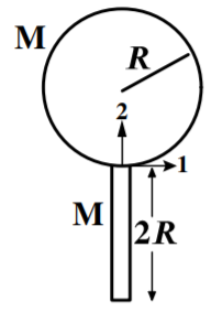
A tennis racquet is an asymmetric body that exhibits the above rotational behavior. Assume that the head of a tennis racquet is a uniform thin circular disk of radius R and mass M which is attached to a cylindrical handle of diameter r=R10, length 2R, and mass M as shown in the figure. The principle moments of inertia about the three axes through the center-of-mass can be calculated by addition of the moments for the circular disk and the cylindrical handle and using both the parallel-axis and the perpendicular-axis theorems.
| Axis | Head | Handle | Racquet |
|---|---|---|---|
| 1 | 14MR2+MR2=54MR2 | 43MR2 | 3112MR2 |
| 2 | 14MR2+0=14MR2 | 1200MR2 | 51200MR2 |
| 3 | 12MR2+MR2=32MR2 | 43MR2 | 176MR2 |
Note that I11:I22:I33=2.5833:0.2550:2.8333. Inserting these principle moments of inertia into equations ???-??? gives the following precession frequencies
Ω1=i0.8976ω1Ω2=0.9056ω2Ω3=0.9892ω3
The imaginary precession frequency Ω1 about the 1 axis implies unstable rotation leading to tumbling whereas the minimum moment I22 and maximum moment I33 imply stable rotation about the 2 and 3 axes. This rotational behavior is easily demonstrated by throwing a tennis racquet and is called the tennis racquet theorem. The center of percussion, example 2.12.8 is another important inertial property of a tennis racquet.
Example 13.22.2: Rotation of asymmetrically-deformed nuclei
Some nuclei and molecules have average shapes that have significant asymmetric deformation leading to interesting quantal analogs of the rotational properties of an asymmetrically-deformed rigid body. The major difference between a quantal and a classical rotor is that the energies, and angular momentum are quantized, rather than being continuously variable quantities. Otherwise, the quantal rotors exhibit general features similar to the classical analog. Studies [Cli86] of the rotational behavior of asymmetrically-deformed nuclei exploit three aspects of classical mechanics, namely classical Coulomb trajectories, rotational invariants, and the properties of ellipsoidal rigid-bodies.
Ellipsoidal deformation can be specified by the dimensions along each of the three principle axes. Bohr and Mottelson parameterized the ellipsoidal deformation in terms of three parameters, R0 which is the radius of the equivalent sphere, β which is a measure of the magnitude of the ellipsoidal deformation from the sphere, and γ which specifies the deviation of the shape from axial symmetry. The ellipsoidal intrinsic shape can be expressed in terms of the deviation from the equivalent sphere by the equation
δR(θ,ϕ)=R(θ,ϕ)−R0=R0μ+2∑μ=−2α∗2μY2μ(θ,ϕ)
where Yλμ(θ,ϕ) is a Laplace spherical harmonic defined as
Yλμ(θ,ϕ)=√(2λ+1)4π(λ−μ)!(λ+μ)!Pλμ(cosθ)e−iμϕ
and Pλμ(cosθ) is an associated Legendre function of cosθ. Spherical harmonics are the angular portion of a set of solutions to Laplace’s equation. Represented in a system of spherical coordinates, Laplace’s spherical harmonics Yλμ(θ,ϕ) are a specific set of spherical harmonics that form an orthogonal system. Spherical harmonics are important in many theoretical and practical applications.
In the principal axis frame of the body, there are three non-zero quadrupole deformation parameters which can be written in terms of the deformation parameters β,γ where α20=βcosγ, α21=α2−1=0, and α22=α2−2=1√2βsinγ. Using these in equations a give the three semi-axis dimensions in the principal axis frame, (primed frame),
δRk=√54πR0βcos(γ−2πk3)
Note that for γ=0, then δR1=δR2=−12√54πR0β while δR3=+√54πR0β, that is the body has prolate deformation with the symmetry axis along the 3 axis. The same prolate shape is obtained for γ=2π3 and γ=4π3 with the prolate symmetry axes along the 1 and 2 axes respectively. For γ=π3 then δR1=δR3=+12√54πR0β while δR2=−√54πR0β, that is the body has oblate deformation with the symmetry axis along the 2 axis. The same oblate shape is obtained for γ=π and γ=5π3 with the oblate symmetry axes along the 3 and 1 axes respectively. For other values of γ the shape is ellipsoidal.
For the asymmetric deformed rigid body, the rotational Hamiltonian can be expressed in the form[Dav58]
H=3∑k=1|R|24Bβ2sin2(γ′−2πk3)
where the rotational angular momentum is R. The principal moments of inertia are related by the triaxiality parameter γ′ which they assumed is identical to the shape parameter γ. For axial symmetry the moment of inertia about the symmetry axis is taken to be zero for a quantal system since rotation of the potential well about the symmetry axis corresponds to no change in the potential well, or corresponding rotation of the bound nucleons. That is, the nucleus is not a rigid body, the nucleons only rotate to the extent that the ellipsoidal potential well is cranked around such that the nucleons must follow the rotation of the potential well. In addition, vibrational modes coexist about the average asymmetric deformation, plus octupole deformation often coexists with the above quadrupole deformed modes.