Physics LibreTexts

13.18: Lagrange equations of motion for rigid-body rotation

  • Page ID
    14190
  • \( \newcommand{\vecs}[1]{\overset { \scriptstyle \rightharpoonup} {\mathbf{#1}} } \) \( \newcommand{\vecd}[1]{\overset{-\!-\!\rightharpoonup}{\vphantom{a}\smash {#1}}} \)\(\newcommand{\id}{\mathrm{id}}\) \( \newcommand{\Span}{\mathrm{span}}\) \( \newcommand{\kernel}{\mathrm{null}\,}\) \( \newcommand{\range}{\mathrm{range}\,}\) \( \newcommand{\RealPart}{\mathrm{Re}}\) \( \newcommand{\ImaginaryPart}{\mathrm{Im}}\) \( \newcommand{\Argument}{\mathrm{Arg}}\) \( \newcommand{\norm}[1]{\| #1 \|}\) \( \newcommand{\inner}[2]{\langle #1, #2 \rangle}\) \( \newcommand{\Span}{\mathrm{span}}\) \(\newcommand{\id}{\mathrm{id}}\) \( \newcommand{\Span}{\mathrm{span}}\) \( \newcommand{\kernel}{\mathrm{null}\,}\) \( \newcommand{\range}{\mathrm{range}\,}\) \( \newcommand{\RealPart}{\mathrm{Re}}\) \( \newcommand{\ImaginaryPart}{\mathrm{Im}}\) \( \newcommand{\Argument}{\mathrm{Arg}}\) \( \newcommand{\norm}[1]{\| #1 \|}\) \( \newcommand{\inner}[2]{\langle #1, #2 \rangle}\) \( \newcommand{\Span}{\mathrm{span}}\)\(\newcommand{\AA}{\unicode[.8,0]{x212B}}\)

    The Euler equations of motion were derived using Newtonian concepts of torque and angular momentum. It is of interest to derive the equations of motion using Lagrangian mechanics. It is convenient to use a generalized torque \(N\) and assume that \(U = 0\) in the Lagrange-Euler equations. Note that the generalized force is a torque since the corresponding generalized coordinate is an angle, and the conjugate momentum is angular momentum. If the body-fixed frame of reference is chosen to be the principal axes system, then, since the inertia tensor is diagonal in the principal axis frame, the kinetic energy is given in terms of the principal moments of inertia as

    \[T = \frac{1}{2} \sum_i I_i \omega^2_i \label{13.104}\]

    Using the Euler angles as generalized coordinates, then the Lagrange equation for the specific case of the \(\psi\) coordinate and including a generalized force \(N_{\psi}\) gives

    \[\frac{d}{dt} \frac{\partial T}{\partial \dot{\psi}} − \frac{\partial T}{\partial \psi} = N_{\psi} \]

    which can be expressed as

    \[\frac{d}{dt} \sum^3_i \frac{\partial T}{\partial \omega_i} \frac{\partial \omega_i}{\partial \dot{\psi}} − \sum^3_i \frac{\partial T}{\partial \omega_i} \frac{\partial \omega_i}{\partial \psi } = N_{\psi} \label{13.106}\]

    Equation \ref{13.104} gives

    \[\frac{\partial T}{\partial \omega_i} = I_i \omega_i\]

    Differentiating the angular velocity components in the body-fixed frame, equations \((13.14.1-13.14.3)\) give

    \(\frac{\partial \omega_1}{\partial \psi} = \dot{\phi} \sin \theta \cos \psi − \dot{\theta} \sin\psi = \omega_2\) \(\frac{\partial \omega_1 }{\partial \dot{\psi}} = \frac{\partial \omega_2}{ \partial \dot{\psi}} = 0\)
    \(\frac{\partial \omega_2 }{\partial \psi} = −\dot{\phi} \sin \theta \sin \psi − \dot{\theta} \cos \psi = −\omega_1\) \(\frac{\partial \omega_1 }{\partial \dot{\psi}} = \frac{\partial \omega_2}{ \partial \dot{\psi}} = 0\)
    \(\frac{\partial \omega_3}{\partial \psi} = 0\) \(\frac{\partial \omega_3 }{\partial \dot{\psi}} = 1\)
    Table \(\PageIndex{1}\)

    Substituting these into the Lagrange Equation \ref{13.106} gives

    \[\frac{d}{dt} I_3\omega_3 − I_1\omega_1\omega_2 + I_2\omega_2 (−\omega_1) = N_3 \]

    since the \(\psi\) and \(\widehat{\mathbf{e}_3}\) axes are colinear. This can be rewritten as

    \[I_3\dot{\omega}_3 − (I_1 − I_2) \omega_1\omega_2 = N_3 \]

    Any axis could have been designated the \(\widehat{\mathbf{e}_3}\) axis, thus the above equation can be generalized to all three axes to give

    \[\begin{align} I_1\dot{\omega}_1 − (I_2 − I_3) \omega_2\omega_3 = N_1 \\ I_2\dot{\omega}_2 − (I_3 − I_1) \omega_3\omega_1 = N_2 \notag \\ I_3\dot{\omega}_3 − (I_1 − I_2) \omega_1\omega_2 = N_3 \notag \end{align}\]

    These are the Euler’s equations given previously in \((13.17.6)\). Note that although \(\dot{\omega}_3\) is the equation of motion for the \(\psi\) coordinate, this is not true for the \(\boldsymbol{\phi}\) and \(\boldsymbol{\theta}\) rotations which are not along the body-fixed \(x_1\) and \(x_2\) axes as given in table \(13.14.1\).

    Example \(\PageIndex{1}\): Rotation of a dumbbell

    11.18.1.PNG
    Figure \(\PageIndex{1}\): Rotation of a dumbbell.

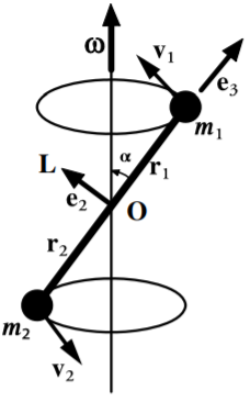
    Consider the motion of the symmetric dumbbell shown in the adjacent figure. Let \(|r_1| = |r_2| = b\). Let the body-fixed coordinate system have its origin at \(O\) and symmetry axis \(\widehat{\mathbf{e}_3}\) be along the weightless shaft toward \(m_1\) and \(\mathbf{v}_{\alpha} = v_{\alpha} \hat{e}_1\). The angular momentum is given by

    \[\mathbf{L} = \sum_i m_i \mathbf{r} \times \mathbf{v}\notag\]

    Because \(\mathbf{L}\) is perpendicular to the shaft, and \(\mathbf{L}\) rotates around \(\boldsymbol{\omega}\) as the shaft rotates, let \(\widehat{\mathbf{e}_2}\) be along \(\mathbf{L}\).

    \[\mathbf{L} = L_2 \widehat{\mathbf{e}_2} \notag\]

    If \(\alpha\) is the angle between \(\boldsymbol{\omega}\) and the shaft, the components of \(\boldsymbol{\omega}\) are

    \[\begin{aligned} \omega_1 = 0 \\ \omega_2 = \omega \sin \alpha \\ \omega_3 = \omega \cos \alpha \end{aligned}\]

    Assume that the principal moments of the dumbbell are

    \[\begin{aligned} I_1 = (m_1 + m_2) b^2 \\ I_2 = (m_1 + m_2) b^2 \\ I_3 = 0 \end{aligned}\]

    Thus the angular momentum is given by

    \[\begin{aligned} L_1 = I_1\omega_1 = 0 \\ L_2 = I_2\omega_2 = (m_1 + m_2) b^2 \omega \sin \alpha \\ L_3 = I_3 \omega_3 = 0 \end{aligned}\]

    which is consistent with the angular momentum being along the \(\widehat{\mathbf{e}_2}\) axis.

    Using Euler’s equations, and assuming that the angular velocity is constant, i.e. \(\dot{\omega}= 0\), then the components of the torque required to satisfy this motion are

    \[\begin{aligned} N_1 = − (m_1 + m_2) b^2 \omega^2 \sin \alpha \cos \alpha \\ N_2 = 0 \\ N_3 = 0 \end{aligned}\]

    That is, this motion can only occur in the presence of the above applied torque which is in the direction \(-\widehat{\mathbf{e}_1}\), that is, mutually perpendicular to \(\widehat{\mathbf{e}_2}\) and \(\widehat{\mathbf{e}_3}\). This torque can be written as \(\mathbf{N} = \boldsymbol{\omega} \times \mathbf{L}\).


    This page titled 13.18: Lagrange equations of motion for rigid-body rotation is shared under a CC BY-NC-SA 4.0 license and was authored, remixed, and/or curated by Douglas Cline via source content that was edited to the style and standards of the LibreTexts platform; a detailed edit history is available upon request.