14.10: Discrete Lattice Chain

Crystalline lattices and linear molecules are important classes of coupled oscillator systems where nearest neighbor interactions dominate. A crystalline lattice comprises thousands of coupled oscillators in a three dimensional matrix with atomic spacing of a few $10^{−10}m$. Even though a full description of the dynamics of crystalline lattices demands a quantal treatment, a classical treatment is of interest since classical mechanics underlies many features of the motion of atoms in a crystalline lattice. The linear discrete lattice chain is the simplest example of many-body coupled oscillator systems that can illuminate the physics underlying a range of interesting phenomena in solid-state physics. As illustrated in example $2.12.1$, the linear approximation usually is applicable for small-amplitude displacements of nearest-neighbor interacting systems which greatly simplifies treatment of the lattice chain. The linear discrete lattice chain involves three independent polarization modes, one longitudinal mode, plus two perpendicular transverse modes. The $3n$ degrees of freedom for the $n$ atoms, on a discrete linear lattice chain, are partitioned with $n$ degrees of freedom for each of the three polarization modes. These three polarization modes each have $n$ normal modes, or $n$ travelling waves, and exhibit quantization, dispersion, and can have a complex wave number.

Longitudinal Motion

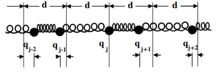
The equations of motion for longitudinal modes of the lattice chain can be derived by considering a linear chain of $n$ identical masses, of mass $m$, separated by a uniform spacing $d$ as shown in Figure $\PageIndex{1}$. Assume that the $n$ masses are coupled by $n + 1$ springs, with spring constant $\kappa$, where both ends of the chain are fixed, that is, the displacements $q_0 = q_{n+1} = 0$ and velocities $\dot{q}_0 = \dot{q}_{n+1} = 0$. The force required to stretch a length $d$ of the chain a longitudinal displacements, $q_{j}$ for mass $j$, is $F_j = \kappa q_j$. Thus the potential energy for stretching the spring for segment $(q_{j−1} − q_j )$ is $U_j = \frac{\kappa}{2} (q_{j-1} - q_j)$. The total potential and kinetic energies are

$$U = \frac{\kappa}{2} \sum^{n+1}_{j=1} (q_{j-1} - q_j)^2 \label{14.74}$$

$$T = \frac{1}{2} m \sum^{n}_{j=1} \dot{q}^2_j \label{14.75}$$

Figure $\PageIndex{1}$: Portion of a lattice chain of identical masses $m$ connected by identical springs of spring constant $\kappa$. The displacement of the $j^{th}$ mass from the equilibrium position is $q_j$ assumed to be positive to the right.

Since $\dot{q}_{n+1} = 0$ the kinetic energy and Lagrangian can be extended to $j = {n+1}$, that is, the Lagrangian can be written as

$$L = \frac{1}{2} \sum^{n+1}_{j=1} \left( m\dot{q}^2_j − \kappa (q_{j−1} − q_j )^2 \right)$$

Using this Lagrangian in the Lagrange-Euler equations gives the following second-order equation of motion for longitudinal oscillations

$$\ddot{q}_j = \omega^2_o (q_{j-1} − 2q_j + q_{j+1}) \label{14.77}$$

where $j = 1, 2, ....n$ and where

$$\omega_o \equiv \sqrt{\frac{\kappa}{m}}$$

Transverse motion

Figure $\PageIndex{2}$: Transverse motion of a linear discrete lattice chain

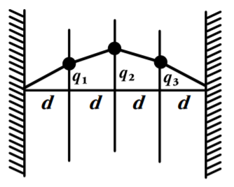
The equations of motion for transverse motion on a linear discrete lattice chain, illustrated in Figure $\PageIndex{2}$, can be derived by considering the displacements $q_j$ of the $i^{th}$ mass for $n$ identical masses, with mass $m$, separated by equal spacings $d$ and assuming that the tension in the string is $r = \left( \frac{\partial U}{\partial x} \right)$. Assuming that the transverse deflections $q_j$ are small, then the $j − 1$ to $j$ spring is stretched to a length

$$d^{\prime} = \sqrt{d^2 + (q_j − q_{j-1})^2}$$

Thus the incremental stretching is

$$\delta d \sim \frac{(q_j − q_{j-1})^2}{2d}$$

The work done against the tension $\tau$ is $\tau \cdot \delta d$ per segment. Thus the total potential energy is

$$U = \frac{\tau}{2d} \sum^{n+1}_{j=1} (q_{j-1} − q_j )^2$$

where $q_0$ and $q_{n+1}$ are identically zero.

The kinetic energy is

$$T = \frac{1}{2} m\sum^n_{ j=1} \dot{q}^2_j$$

Since $\dot{q}_{n+1} = 0$, the kinetic energy and Lagrangian summations can be extended to $j = n + 1$, that is

$$L = \frac{1}{2} \sum^{n+1}_{j=1} \left( m\dot{q}^2_j − \frac{\tau}{d} (q_{j-1} − q_j )^2 \right)$$

Using this Lagrangian in the Lagrange Euler equations gives the following second-order equation of motion for transverse oscillations

$$\ddot{q}_j = \omega^2_o (q_{j-1} − 2q_j + q_{j+1}) \label{14.84}$$

where $j = 1, 2, ....n$ and

$$\omega_o \equiv \sqrt{\frac{\tau}{dm}}$$

The normal modes for the transverse modes comprise standing waves that satisfy the same boundary conditions as for the longitudinal modes. The $n$ equations of motion for longitudinal motion, Equation $\ref{14.77}$, or transverse motion, Equation $\ref{14.84}$, are identical in form. The major difference is that $\omega_0$ for the transverse normal modes $\omega_o \equiv \sqrt{\frac{\tau}{dm}}$ differs from that for the longitudinal modes which is $\omega_o \equiv \sqrt{\frac{\kappa}{m}}$. Thus the following discussion of the normal modes on a discrete lattice chain is identical in form for both transverse and longitudinal waves.

Normal modes

The normal modes of the $n$ equations of motion on the discrete lattice chain, are either longitudinal or transverse standing waves that satisfy the boundary conditions at the extreme ends of the lattice chain. The solutions can be given by assuming that the $n$ identical masses on the chain oscillate with a common frequency $\omega$. Then the displacement amplitude for the $j^{th}$ mass can be written in the form

$$q_j (t) = a_j e^{i\omega t}$$

where the amplitude $a_j$ can be complex. Substitution into the preceding $n$ equations of motion, $\ref{14.77}$, $\ref{14.84}$, yields the following recursion relation

$$\left( −\omega^2 + 2\omega^2_o \right) a_j− \omega^2_0 (a_{j−1} + a_{j+1})=0 \label{14.87}$$

where $j = 1, 2, ...n$. Note that the boundary conditions, $q_0 = 0$ and $q_{n+1} = 0$ require that $a_o = a_{n+1} = 0$.

The above recursion relation corresponds to a system of $n$ homogeneous algebraic equations with $n$ unknowns $a_1, a_2, ...a_n$. A non-trivial solution is given by setting the determinant of its coefficients equal to zero

$$\begin{vmatrix} −\omega^2 + 2\omega^2_o & −\omega^2_o & 0 & 0 \\ −\omega^2_o & −\omega^2 + 2\omega^2_o & −\omega^2_o & 0 \\ 0 & −\omega^2_o & −\omega^2 + 2\omega^2_o & −\omega^2_o \\ ..... & .... & ..... & ..... \\ 0 & 0 & −\omega^2_o & −\omega^2 + 2\omega^2_o \end{vmatrix} = 0$$

This secular determinant corresponds to the special case of nearest neighbor interactions with the kinetic energy tensor $\mathbf{T}$ being diagonal and the potential energy tensor $\mathbf{V}$ involving coupling only to adjacent masses. The secular determinant is of order $n$ and thus determines exactly $n$ eigen frequencies $\omega_r$ for each polarization mode.

For large $n$, the solution of this problem is more efficiently obtained by using a recursion relation approach, rather than solving the above secular determinant. The trick is to assume that the phase differences $\phi_r$ between the motion of adjacent masses all are identical for a given polarization. Then the amplitude for the $j^{th}$ mass for the $r^{th}$ frequency mode $\omega_r$ is of the form

$$a_{jr} = a_{r} e^{i(j\phi_r−\delta_r)}$$

Insert the above into the recursion relation $\ref{14.87}$ gives

$$\left( −\omega^2_r + 2\omega^2_o \right) − \omega^2_0 \left[ e^{-i\phi_r} + e^{i\phi_r} \right] = 0$$

which reduces to

$$\omega^2_r = 2\omega^2_o − 2\omega^2_o \cos \phi_r = 4\omega^2_o \sin^2 \frac{\phi_r}{2}$$

that is

$$\omega_r = 2\omega_o \sin \frac{\phi_r}{2}$$

where $r = 1, 2, 3, ....n$.

Now it is necessary to determine the phase angle $\phi_r$ which can be done by applying the boundary conditions for standing waves on the lattice chain. These boundary conditions for stationary modes require that the ends of the lattice chain are nodes, that is $a_{o,r} = a_{(n+1),r} = 0$. Using the fact that only the real part of $a_{jr}$ has physical meaning, leads to the amplitude for the $j^{th}$ mass for the $r^{th}$ mode to be

$$a_{j,r} = a_{r} \cos (j\phi_r − \delta_r)$$

The boundary condition $a_{0r} = 0$ requires that the phase $\delta_r = \frac{\pi}{2}$. That is

$$a_{jr} = a_{r} \cos \left( j\phi_r − \frac{\pi }{2} \right) = a_{r} \sin j\phi_r \label{14.93}$$

where $r = 1, 2, ..., n$.

The boundary condition for $j = n+1$, gives

$$a_{(n+1)r} =0= a_{r} \sin (n+1) \phi_r$$

Therefore

$$(n+1) \phi_r = r\pi$$

where $r = 1, 2, 3, ..., n$. That is

$$\phi_r = \frac{r\pi}{n+1} = \frac{r\pi d}{ (n+1) d} = \frac{r\pi d}{D} = \frac{k_r d}{2} \label{14.96}$$

where $D = (n+1)d$ is the total length of the discrete lattice chain.

The $n$ eigen frequencies for a given polarization are given by

$$\omega_r = 2\omega_o \sin \frac{r\pi}{ 2 (n+1)} = 2\omega_o \sin \frac{r\pi d}{2 (n+1) d} = 2\omega_o \sin\frac{ r\pi d}{ 2D} = 2\omega_o \sin \frac{k_rd}{ 2} \label{14.97}$$

where the corresponding wavenumber $k_r$ is given by

$$k_r = \frac{r\pi }{(n+1) d }= \frac{r\pi}{D} = \frac{2\pi}{ \lambda_r}$$

This implies that the normal modes are quantized with half-wavelengths $\frac{\lambda_r}{2} = \frac{D}{r}$.

Figure $\PageIndex{3}$: Plots of the maximal vibrational amplitudes $a_r$ for the $r^{th}$ frequency sinusoidal mode, versus distance along the chain, for transverse normal modes of a vibrating discrete lattice with $n = 5$. Only $r = 1, 2, 3, 4, 5,$ are distinct modes because $r = 6$ is a null mode. Note that the modes with $r = 7, 8, 9, 10, 11, 12,$ shown dashed, duplicate the locations of the mass displacement given by the lower-order modes.

Combining equations $\ref{14.96}$ and $\ref{14.93}$ gives the maximum amplitudes for the eigenvectors to be

$$a_{jr} = a_r \sin j \frac{k_r d}{2} \label{14.99}$$

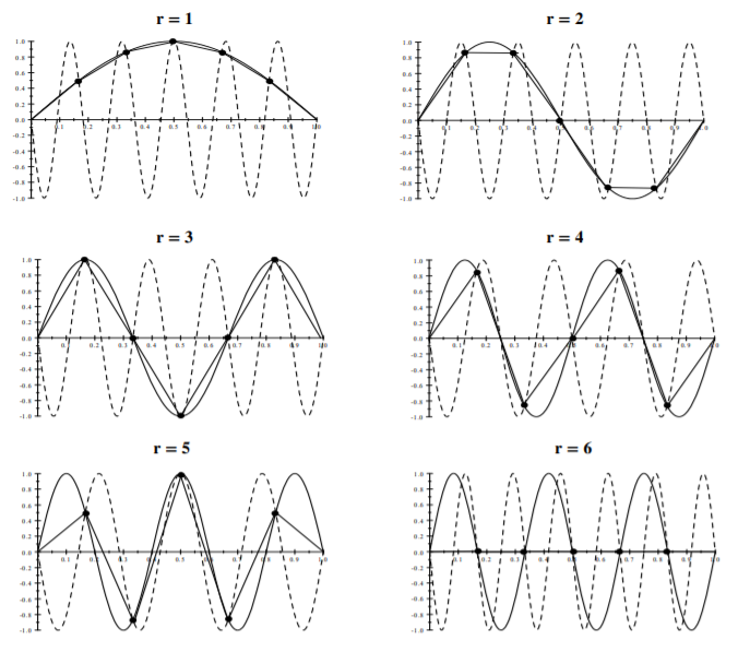
For $n$ independent linear oscillators there are only $n$ independent normal modes, that is, for $r = n+1$ the sine function in Equation $\ref{14.97}$ must be zero. Beyond $r = n$ the equations do not describe physically new situations. This is illustrated by Figure $\PageIndex{3}$ which shows the transverse modes of a lattice chain with $n = 5$. There are only $n = 5$ independent normal modes of this system since $r = n +1=6$ corresponds to a null mode with all $q_j (t)=0$. Also note that the solutions for $r>n+1$, shown dashed, replicate the mass locations of modes with $r<n+1$, that is, the modes with $r > 6$ are replicas of the lower-order modes.

Note that $\omega_r$ has a maximum value $\omega_r \leq 2\omega_0$ since the sine function cannot exceed unity. This leads to a maximum frequency $\omega_c = 2\omega_0$, called the cut-off frequency, which occurs when $k_rd = \pi$. That is, the null-mode occurs when $r = n+1$ for which Equation $\ref{14.99}$ equals zero. The range of $n$ quantized normal modes that can occur is intuitive. That is, the longest half-wavelength $\frac{\lambda_{\text{max}}}{2} = D = ({n+1})d$ equals the total length of the discrete lattice chain. The shortest half-wavelength $\frac{\lambda_{cut−off}}{2} = d$ is set by the lattice spacing. Thus the discrete wavenumbers of the normal modes, for each polarization, range from $k_1$ to $nk_1$ where $n$ is an integer.

Assuming real $k_r$, the normal coordinate $\eta_r$ and corresponding frequency $\omega_r$ are,

$$\eta_r = a_{r} e^{i\omega_rt}$$

Equations $\ref{14.97}$ and $\ref{14.99}$ give the angular frequency and displacement. Note that superposition applies since this system is linear. Therefore the most general solution for each polarization can be any superposition of the form

$$q_j (t) = \sum^n_{ r=1 } \eta_r \sin \left[ \frac{r\pi j}{ (n+1)} \right]$$

Travelling waves

Travelling waves are equally good solutions of the equations of motion $\ref{14.77}$, $\ref{14.84}$ as are the normal modes. Travelling waves on the one-dimensional lattice chain will be of the form

$$q (x, t) = Ce^{i(\omega t \pm kx)} \label{14.102}$$

where the distance along the chain $x = \nu d$, that is, it is quantized in units of the cell spacing $d$, with $\nu$ being an integer. The positive sign in the exponent corresponds to a wave travelling in the $−x$ direction while the negative sign corresponds to a wave travelling in the $+x$ direction. The velocity of a fixed phase of the travelling wave must satisfy that $\omega t \pm kx$ is a constant. This will occur if the phase velocity of the wave is given by

$$v^{phase} = \frac{dx}{dt} = \frac{\omega}{k}$$

The wave has a frequency $f = \frac{\omega}{ 2\pi}$ and wavelength $\lambda = \frac{2\pi}{k}$, thus the phase velocity $v_{phase} = \frac{\omega}{k} = \lambda f$.

Inserting the travelling wave $\ref{14.102}$ into the transverse equation of motion $\ref{14.84}$ for the discrete lattice chain gives

$$−\omega^2q_r = \omega^2_0(e^{−\phi_r} − 2 + e^{\phi_r} )q_r$$

where $j = 1, 2, ....n$. That is

$$\omega_r = \pm 2\omega_0 \sin \frac{\phi_r}{2} \label{14.105}$$

The phase $\phi_r$ is determined by the Born-von Karman periodic boundary condition that assumes that the chain is duplicated indefinitely on either side of $k = \pm \frac{\pi}{d}$. Thus, for $n$ discrete masses, $k$ must satisfy the condition that $q_r = q_{r+n}$. That is

$$e^{ik_rnd} = 1$$

That is

$$k_r = \frac{2\pi r}{nd}$$

Note that the periodic boundary condition gives $n$ discrete modes for wavenumbers between

$$−\frac{\pi}{d} \leq k_r \leq + \frac{\pi}{d}$$

where the index

$$r = −\frac{n}{2}, −\frac{n}{2} + 1, ....., \frac{n}{2} − 1, \frac{n}{2} \nonumber$$

Thus Equation $\ref{14.105}$ becomes

$$\omega_r = \pm 2\omega_0 \sin \frac{k_r d}{2} \label{14.109}$$

Equation $\ref{14.109}$ is a dispersion relation that is identical to Equation $\ref{14.97}$ derived during the discussion of the normal modes of the lattice chain. This confirms that the travelling waves on the lattice chain are equally good solutions as the normal standing-wave modes. Clearly, superposition of the standing-wave normal modes can lead to travelling waves and vice versa.

Dispersion

Figure $\PageIndex{4}$: Plot of the dispersion curve ($\omega$ versus $k$) for a monoatomic linear lattice chain subject to only nearest neighbor interactions. The first Brillouin zone is the segment between $−\frac{\pi}{d} \leq k \leq \frac{\pi}{d}$ which covers all independent solutions.

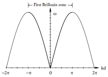
The lattice chain is an interesting example of a dispersive system in that $\omega_r$ is a function of $k_r$. Figure $\PageIndex{4}$ shows a plot of the dispersion curve ($\omega$ versus $k$) for a monoatomic linear lattice chain subject to only nearest neighbor interactions. Note that $\omega$ depends linearly on $k$ for small $k$ and that $\frac{d\omega}{dk} = 0$ at the boundaries of the first Brillouin zone.

The lattice chain has a phase velocity for the $r^{th}$ wave given by

$$v^{phase}_r = \frac{\omega_r}{k_r} = \omega_0 d \frac{|\sin \frac{k_r d}{2}|}{ \frac{k_r d}{2}}$$

while the group velocity is

$$v^{group}_r = \left(\frac{d\omega}{dk} \right)_r = \omega_0 d \cos \frac{k_r d}{2}$$

Note that in the limit when $\frac{k_r d}{2} \rightarrow 0$, the phase velocity and group velocity are identical, that is, $v^{phase}_r = v^{group}_r = \omega_0d$.

Complex wavenumber

The maximum allowed frequency, which is called the cut-off frequency, $\omega_c = 2\omega_0$, occurs when $k_rd = \pi$, that is, $\frac{\lambda}{2} = d$. That is, the minimum half-wavelength equals the spacing $d$ between the discrete masses. At the cut-off frequency, the phase velocity is $v^{phase}_r = \frac{2}{\pi } \omega_0d$ and the group velocity $v^{group}_r = 0$.

It is interesting to note that $\omega_r$ can exceed the cut-off frequency $\omega_c = 2\omega_0$ if $k_r$ is assumed to be complex, that is, if

$$k_r = \kappa_r − i\Gamma_r$$

Then

$$\omega_r = 2\omega_0 \sin \frac{k_r d}{2} = 2\omega_0 \sin \frac{d}{2} (\kappa_r − i\Gamma_r)=2\omega_0 \left( \sin \frac{\kappa_rd}{2} \cosh \frac{\Gamma_rd}{2} − i \cos \frac{\kappa_rd}{2} \sinh \frac{\Gamma_rd }{2} \right)$$

To ensure that $\omega_r$ is real, the imaginary term must be zero, that is

$$\cos \frac{\kappa_rd}{2} = 0$$

Therefore

$$\sin \frac{\kappa_rd}{2} = 1$$

that is, $k_r = \frac{\pi}{d}$, and the dispersion relation between $\omega$ and $k$ for $\omega > 2\omega_0$ becomes

$$\omega_r = 2\omega_0 \cosh \frac{\Gamma_rd}{2}$$

which increases with $\Gamma$. Thus, when $\omega > \omega_c = 2\omega_0$ then the amplitude of the wave is of the form

$$q_r (t) = a_r e^{−\Gamma_rx}e^{i(\omega_rt−\kappa_rx)}$$

which corresponds to a spatially damped oscillatory wave with phase velocity

$$v^{phase}_r = \frac{\omega_r}{\kappa_r}$$

and damping factor $\Gamma_r$.

There are many examples in physics where the wavenumber is complex as exhibited by the discrete lattice chain for $\frac{\lambda}{2} \leq d$. Other examples are electromagnetic waves in conductors or plasma (example $3.11.3$), matter waves tunnelling through a potential barrier, or standing waves on musical instruments which have a complex wavenumber $k$ due to damping.

This simple toy model of the discrete linear lattice chain has illustrated that classical mechanics explains many features of the many-body nearest-neighbor coupled linear oscillator system, including normal modes, standing and travelling waves, cut-off frequency dispersion, and complex wavenumber. These phenomena feature prominently in applications of the quantal discrete coupled-oscillator system to solid-state physics.