14.2: Two Coupled Linear Oscillators

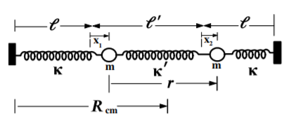
Consider the two-coupled linear oscillator, shown in Figure \(\PageIndex{1}\), which comprises two identical masses each connected to fixed locations by identical springs having a force constant \(\kappa\). A spring with force constant \(\kappa^{\prime}\) couples the two oscillators. The equilibrium lengths of the outer two springs are \(l\) while that of the coupling spring is \(l^{\prime}\). The problem is simplified by restricting the motion to be along the line connecting the masses and assuming fixed endpoints. The small displacements of \(m_1\) and \(m_2\) are taken to be \(x_1\) and \(x_2\) with respect to the equilibrium positions \(l\) and \(l + l^{\prime}\) respectively. The restoring force on \(m_1\) is \(−\kappa x_1−\kappa^{\prime} (x_1 − x_2)\) while the restoring force on \(m_2\) is \(−\kappa x_2 − \kappa^{\prime} (x_2 − x_1)\). This coupled double-oscillator system exhibits basic features of coupled linear oscillator systems.

Figure \(\PageIndex{1}\): Two coupled linear oscillators. The equilibrium spring-lengths are \(l\) for the outer springs and \(l^{\prime}\) for the coupling spring. The displacement from the stable locations are given by \(x_1\) and \(x_2\). The separation between the two masses is \(r\) and the location of the center-of-mass is \(R_{cm}\).

Assuming \(m_1 = m_2 = m\), then the equations of motion are

\[\begin{align} m\ddot{x}_1 + (\kappa + \kappa^{\prime} ) x_1 − \kappa^{\prime} x_2 = 0 \label{14.1} \\ \notag m\ddot{x}_2 + (\kappa + \kappa^{\prime} ) x_2 − \kappa^{\prime} x_1 = 0 \notag\end{align} \]

Assume that the motion for these coupled equations is oscillatory with a solution of the form

\[\begin{align} x_1 = B_1 e^{i\omega t} \label{14.2}\\ x_2 = B_2e^{i\omega t} \notag\notag\end{align}\]

where the constants \(B\) may be complex to take into account both the magnitude and phase. Substituting these possible solutions into the equations of motion gives

\[\begin{align} −m\omega^2 B_1 e^{i\omega t} + (\kappa + \kappa^{\prime} ) B_1e^{i\omega t} − \kappa^{\prime} B_2e^{i\omega t} = 0 \label{14.3}\\ −m\omega^2B_2 e^{i\omega t} + (\kappa + \kappa^{\prime} ) B_2e^{i\omega t} − \kappa^{\prime} B_1 e^{i\omega t} = 0 \notag\end{align}\]

Collecting terms, and cancelling the common exponential factor, gives

\[\begin{align} (\kappa + \kappa^{\prime} − m\omega^2) B_1 − \kappa^{\prime} B_2 = 0 \label{14.4} \\ ( \kappa + \kappa^{\prime} − m\omega^2 ) B_2 − \kappa^{\prime} B_1 = 0 \notag\end{align}\]

The existence of a non-trivial solution of these two simultaneous equations requires that the determinant of the coefficients of \(B_1\) and \(B_2\) must vanish, that is

\[\begin{vmatrix} \kappa + \kappa^{\prime} − m\omega^2 & −\kappa^{\prime} \\ −\kappa^{\prime} & \kappa + \kappa^{\prime} − m\omega^2 \end{vmatrix} = 0 \label{14.5}\]

The expansion of this secular determinant yields

\[( \kappa + \kappa^{\prime} − m\omega^2 )^2 − \kappa^{\prime 2} = 0 \label{14.6}\]

Solving for \(\omega\) gives

\[\omega = \sqrt{\frac{\kappa + \kappa^{\prime} \pm \kappa^{\prime}}{m}} \label{14.7}\]

That is, there are two characteristic frequencies (or eigenfrequencies) for the system

\[\omega_1 = \sqrt{\frac{\kappa + 2\kappa^{\prime} }{m}} \label{14.8}\]

\[\omega_2 = \sqrt{\frac{\kappa}{m}} \label{14.9}\]

Since superposition applies for these linear equations, then the general solution can be written as a sum of the terms that account for the two possible values of \(\omega\).

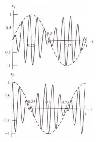
Figure \(\PageIndex{2}\): Displacement of each of two coupled linear harmonic oscillators with \(\kappa = 4\) and \(\kappa^{\prime} = 1\) in relative units.

Figure \(\PageIndex{2}\) shows the solutions for a case where \(\kappa = 4\) and \(\kappa^{\prime} = 1\), in arbitrary units, with the initial condition that \(x_2 = D\), and \(x_1 = \dot{x}_1 = \dot{x}_2 = 0\). The two characteristic frequencies are \(\omega_1 = \sqrt{\frac{6}{m}}\) and \(\omega_2 = \sqrt{\frac{4}{m}}\). The characteristic beats phenomenon is exhibited where the envelope over one complete cycle of the low frequency encompasses several higher frequency oscillations. That is, the solution is

\[x_{2}(t)=\frac{D}{4}\left[e^{i \omega_{1} t}+e^{-i \omega_{1} t}+e^{i \omega_{2} t}+e^{-i \omega_{2} t}\right]=D \cos \left[\left(\frac{\omega_{1}+\omega_{2}}{2}\right) t\right] \cos \left[\left(\frac{\omega_{1}-\omega_{2}}{2}\right) t\right] \]

while

\[x_{1}(t)=\frac{D}{4}\left[e^{i \omega_{1} t}+e^{-i \omega_{1} t}-e^{i \omega_{2} t}-e^{-i \omega_{2} t}\right]=D \sin \left[\left(\frac{\omega_{1}+\omega_{2}}{2}\right) t\right] \sin \left[\left(\frac{\omega_{1}-\omega_{2}}{2}\right) t\right]\]

The energy in the two-coupled oscillators flows back and forth between the coupled oscillators as illustrated in Figure \(\PageIndex{2}\).

A better understanding of the energy flow occurring between the two coupled oscillators is given by using a \((x_1, x_2)\) configuration-space plot, shown in Figure \(14.3.1\). The flow of energy occurring between the two coupled oscillators can be represented by choosing normal-mode coordinates \(\eta_1\) and \(\eta_2\) that are rotated by \(45^{\circ}\) with respect to the spatial coordinates \((x_1, x_2)\). These normal-mode coordinates \((\eta_1, \eta_2)\) correspond to the two normal modes of the coupled double-oscillator system.