15.2: Poisson bracket Representation of Hamiltonian Mechanics

Poisson Brackets

Poisson brackets were developed by Poisson, who was a student of Lagrange. Hamilton’s canonical equations of motion describe the time evolution of the canonical variables \((q,p)\) in phase space. Jacobi showed that the framework of Hamiltonian mechanics can be restated in terms of the elegant and powerful Poisson bracket formalism. The Poisson bracket representation of Hamiltonian mechanics provides a direct link between classical mechanics and quantum mechanics.

The Poisson bracket of any two continuous functions of generalized coordinates \(F(p, q)\) and \(G(p, q)\), is defined to be

\[\{F,G\}_{qp} \equiv \sum_i \left(\frac{\partial F}{\partial q_i} \frac{\partial G} {\partial p_i} − \frac{\partial F} {\partial p_i }\frac{\partial G} {\partial q_i} \right) \label{15.12}\]

Note that the above definition of the Poisson bracket, written using the common brace notation, leads to the following identity, antisymmetry, linearity, Leibniz rules, and Jacobi Identity.

\[\begin{align} \{F, F\} &= 0 \\[4pt] \{F,G\}  &= − \{G, F\} \\[4pt]  \{G, F + Y \} &= \{G, F\}+\{G, Y \} \\[4pt]  \{G, F Y \} &= \{G, F\} Y + F \{G, Y \} \\[4pt] 0 &= \{F, \{G, Y \}\} + \{G, \{Y,F\}\} + \{Y \{F,G\}\} \label{15.17} \end{align}\]

where \(G\), \(H\), and \(Y\) are functions of the canonical variables plus time. Jacobi’s identity; \ref{15.17} states that the sum of the cyclic permutation of the double Poisson brackets of three functions is zero. Jacobi’s identity plays a useful role in Hamiltonian mechanics as will be shown.

Fundamental Poisson Brackets

The Poisson brackets of the canonical variables themselves are called the fundamental Poisson brackets. They are

\[ \{q_k, q_l\}_{qp} = \sum_i \left(\frac{\partial q_k}{ \partial q_i} \frac{\partial q_l}{\partial p_i} − \frac{\partial q_k}{ \partial p_i} \frac{\partial q_l}{ \partial q_i} \right) = \sum_i (\delta_{ki} \cdot 0 − 0 \cdot \delta_{li}) = 0 \]

\[ \{p_k, p_l\}_{qp} = \sum_i \left(\frac{\partial p_k }{\partial q_i} \frac{\partial p_l}{ \partial p_i} − \frac{\partial p_k }{\partial p_i} \frac{\partial p_l}{ \partial q_i } \right) = \sum_i (0 \cdot \delta_{li} − \delta_{ki} \cdot 0) = 0 \]

\[ \{q_k, p_l\}_{qp} = \sum_i \left(\frac{\partial q_k}{ \partial q_i} \frac{\partial p_l}{ \partial p_i} − \frac{\partial q_k}{ \partial p_i} \frac{\partial p_l}{ \partial q_i} \right) = \sum_i (\delta_{ki} \cdot \delta_{li} − 0 \cdot 0) = \delta_{kl} \]

In summary, the fundamental Poisson brackets equal

\[ \{q_k, q_l\}_{qp} = 0 \]

\[ \{p_k, p_l\}_{qp} = 0 \]

\[ \{q_k, p_l\}_{qp} = − \{p_l, q_k\}_{qp} = \delta_{kl} \]

Note that the Poisson bracket is antisymmetric under interchange in \(p\) and \(q\). It is interesting that the only non-zero fundamental Poisson bracket is for conjugate variables where \(k = l\), that is

\[ \{q_k, p_k\}_{pq} = 1 \]

Poisson bracket invariance to canonical transformations

The Poisson brackets are invariant under a canonical transformation from one set of canonical variables \((q_k, p_k)\) to a new set of canonical variables \((Q_k, P_k)\) where \(Q_k \rightarrow Q_k(\mathbf{q}, \mathbf{p})\) and \(P_k \rightarrow P_k(\mathbf{q}, \mathbf{p})\). This is shown by transforming Equation \ref{15.12} to the new variables by the following derivation

\[\begin{align} \{F,G\}_{qp} & = \sum_{j} \left( \frac{\partial F}{ \partial q_j} \frac{\partial G} {\partial p_j} − \frac{\partial F} {\partial p_j} \frac{\partial G} {\partial q_j} \right) \label{15.25} \\[4pt] & = \sum_{jk} \left( \frac{\partial F}{ \partial q_j }\left( \frac{\partial G}{ \partial Q_k }\frac{\partial Q_k }{\partial p_j} + \frac{\partial G} {\partial P_k }\frac{\partial P_k}{ \partial p_j} \right) − \frac{\partial F}{ \partial p_j} \left( \frac{\partial G} {\partial Q_k} \frac{\partial Q_k}{ \partial q_j} + \frac{\partial G}{ \partial P_k }\frac{\partial P_k} {\partial q_j} \right)\right) \label{15.26}\end{align}\]

The terms can be rearranged to give

\[ \{F,G\}_{qp} = \sum_k \left( \frac{\partial G}{ \partial Q_k} \{F, Q_k\}_{qp} + \frac{\partial G}{ \partial P_k} \{F, P_k\}_{qp}\right) \label{15.27}\]

Let \(F = Q_k\) and replace \(G\) by \(F\), and use the fact that the fundamental Poisson brackets \(\{Q_k, Q_j \}_{qp} = 0\) and \(\{Q_k, P_j \}_{qp} = \delta_{jk}\), then Equation \ref{15.25} reduces to

\[ \{Q_k, F\}_{qp} = \sum_j \left( \frac{\partial F}{ \partial Q_j} \{Q_k, Q_j \} + \frac{\partial F} {\partial P_j } \{Q_k, P_j \} \right) = \sum_j \frac{\partial F}{ \partial P_j} \delta_{jk} \]

That is

\[ \{F, Q_k\} = − \frac{\partial F} {\partial P_k} \label{15.29}\]

Similarly

\[ \{P_k, F\}_{qp} = \sum_j \left( \frac{\partial F}{ \partial Q_j} \{P_k, Q_j \}_{qp} + \frac{\partial F}{ \partial P_j} \{P_k, P_j \}_{qp} \right) \]

leading to

\[ \{F, P_k\}_{qp} = \frac{\partial F} {\partial Q_k} \label{15.31}\]

Substituting equations \ref{15.29} and \ref{15.31} into Equation \ref{15.27} gives

\[ \{F,G\}_{qp} = \sum_k \left( \frac{\partial F} {\partial Q_k} \frac{\partial G}{ \partial P_k} − \frac{\partial F} {\partial P_k} \frac{\partial G} {\partial Q_k} \right) = \{F,G\}_{QP} \]

Thus the canonical variable subscripts \((q,p)\) and \((Q,P)\) can be ignored since the Poisson bracket is invariant to any canonical transformation of canonical variables. The counter argument is that if the Poisson bracket is independent of the transformation, then the transformation is canonical.

Example \(\PageIndex{1}\): Check that a transformation is canonical

The independence of Poisson brackets to canonical transformations can be used to test if a transformation is canonical. Assume that the transformation equations between two sets of coordinates are given by

\[Q = \ln \left( 1 + q^{\frac{1}{2}} \cos p \right) \quad P = 2 \left( 1 + q^{\frac{1}{2}} \cos p \right) q^{\frac{1}{2}} \sin p \nonumber\]

Evaluating the Poisson brackets gives \(\{Q, Q\} = 0\), \(\{P, P\} = 0\) while

\[\begin{aligned} \{Q, P\} & = \frac{\partial Q}{ \partial q} \frac{\partial P}{ \partial p} − \frac{\partial P}{ \partial q} \frac{\partial Q}{ \partial p} \\ & = \frac{q^{−\frac{ 1}{ 2}} \cos p}{ 1 + q^{\frac{1}{2}} \cos p} [−q \sin^2 p + (1 + q^{\frac{1}{2}} \cos p) q^{\frac{1}{2}} \cos p] + \frac{q^{\frac{1}{2}} \sin^2 p}{ 1 + q^{\frac{1}{2}} \cos p } [\cos p + (1 + q^{\frac{1}{2}} \cos p) q^{− \frac{1}{ 2}} ] = 1 \end{aligned}\]

Therefore if \(q, p\) are canonical with a Poisson bracket \(\{q, p\} = 1\), then so are \(Q, P\) since \(\{Q, P\} = 1 = \{q, p\}\).

Since it has been shown that this transformation is canonical, it is possible to go further and determine the function that generates this transformation. Solving the transformation equations for \(q\) and \(p\) give

\[q = \left( e^Q − 1 \right)^2 \sec^2 p \quad P = 2e^Q \left( e^Q − 1 \right) \tan p \nonumber\]

Since the transformation is canonical, there exists a generating function \(F_3 (Q, p)\) such that

\[q = −\frac{\partial F_3}{ \partial p} \quad P = −\frac{\partial F_3}{ \partial Q} \nonumber\]

The transformation function \(F_3 (Q, p)\) can be obtained using

\[\begin{aligned} dF_3(Q, p) = \frac{\partial F_3}{ \partial Q} dQ + \frac{\partial F_3}{ \partial p }dp = −P dQ − qdp \\ = −d \left[\left( e^Q − 1 \right)^2 \right] \tan p − \left( e^Q − 1 \right)^2 d \tan p = −d \left[\left( e^Q − 1 \right)^2 \tan p \right] \end{aligned}\]

This then gives that the required generating function is

\[F_3(Q, p) = \left( e^Q − 1 \right)^2 \tan p \nonumber\]

This example illustrates how to determine a useful generating function and prove that the transformation is canonical.

Correspondence of the Commutator and the Poisson Bracket

In classical mechanics there is a formal correspondence between the Poisson bracket and the commutator. This can be shown by deriving the Poisson Bracket of four functions taken in two pairs. The derivation requires deriving the two possible Poisson Brackets involving three functions.

\[ \begin{align} \{F_1F_2, G\} & = \sum_j \left[ \left(\frac{\partial F_1}{ \partial q_j } F_2 + F_1 \frac{\partial F_2}{ \partial q_j} \right) \frac{\partial G} {\partial p_j} − \left(\frac{\partial F_1}{ \partial p_j} F_2 + F_1 \frac{\partial F_2}{ \partial p_j} \right) \frac{\partial G}{ \partial q_j} \right] \\[4pt] &= \{F_1, G\} F_2 + F_1 \{F_2, G\} \label{15.33} \end{align}\]

\[ \{F,G_1G_2\} = \{F,G_1\} G_2 + G_1 \{F,G_2\} \label{15.34}\]

These two Poisson Brackets for three functions can be used to derive the Poisson Bracket of four functions, taken in pairs. This can be accomplished two ways using either Equation \ref{15.33} or \ref{15.34}.

\[ \{F_1F_2, G_1G_2\} = \{F_1, G_1G_2\} F_2 + F_1 \{F_2, G_1G_2\} \\ = [ \{F_1, G_1\} G_2 + G_1 \{F_1, G_2\} ] F_2 + F_1 [\{F_2, G_1\} G_2 + G_1 \{F_2, G_2\}] \\ = \{F_1, G_1\} G_2F_2 + G_1 \{F_1, G_2\} F_2 + F_1 \{F_2, G_1\} G_2 + F_1G_1 \{F_2, G_2\} \label{15.35}\]

The alternative approach gives

\[ \{F_1F_2, G_1G_2\} = \{F_1F_2,G_1\} G_2 + G_1 \{F_1F_2, G_2\} \\ = \{F_1, G_1\} F_2G_2 + F_1 \{F_2, G_1\} G_2 + G_1 \{F_1, G_2\} F_2 + G_1F_1 \{F_2, G_2\} \label{15.36}\]

These two alternate derivations give different relations for the same Poisson Bracket. Equating the alternative equations \ref{15.35} and \ref{15.36} gives that

\[ \{F_1, G_1\} (F_2G_2 − G_2F_2) = (F_1G_1 − G_1F_1) \{F_2, G_2\} \nonumber\]

This can be factored into separate relations, the left-hand side for body 1, and the right-hand side for body 2.

\[\frac{(F_1G_1 − G_1F_1)}{ \{F_1, G_1\}} = \frac{(F_2G_2 − G_2F_2)}{ \{F_2, G_2\} } = \lambda \]

Since the left-hand ratio holds for \(F_1, G_1\) independent of \(F_2, G_2\), and vise versa, then they must equal a constant \(\lambda\) that does not depend on \(F_1, G_1\), does not depend on \(F_2, G_2\), and \(\lambda\) must commute with \((F_1G_1 − G_1F_1)\). That is, \(\lambda\) must be a constant number independent of these variables.

\[(F_1G_1 − G_1F_1) = \lambda \{F_1, G_1\} \equiv \lambda \sum_i \left(\frac{\partial F_1}{ \partial q_i} \frac{\partial G_1 }{\partial p_i} − \frac{\partial F_1 }{\partial p_i }\frac{\partial G_1}{ \partial q_i} \right) \label{15.38}\]

Equation \ref{15.38} is an especially important result which states that to within a multiplicative constant number \(\lambda\), there is a one-to-one correspondence between the Poisson Bracket and the commutator of two independent functions. An important implication is that if two functions, \(F_iG_k\) have a Poisson Bracket that is zero, then the commutator of the two functions also must be zero, that is, \(F_i\) and \(G_k\) commute.

Consider the special case where the variables \(F_1\) and \(G_1\) correspond to the fundamental canonical variables, \((q_k, p_l)\). Then the commutators of the fundamental canonical variables are given by

\[q_kp_l − p_lq_k = \lambda \{q_k, p_l\} = \lambda\delta_{kl} \]

\[q_kq_l − q_lq_k = \lambda \{q_k, q_l\} = 0 \]

\[p_kp_l − p_lp_k = \lambda \{p_k, p_l\} = 0 \]

In 1925, Paul Dirac, a 23-year old graduate student at Bristol, recognized that the formal correspondence between the Poisson bracket in classical mechanics, and the corresponding commutator, provides a logical and consistent way to bridge the chasm between the Hamiltonian formulation of classical mechanics, and quantum mechanics. He realized that making the assumption that the constant \(\lambda \equiv i\hbar\), leads to Heisenberg’s fundamental commutation relations in quantum mechanics, as is discussed in chapter \(18.3.1\). Assuming that \(\lambda \equiv i\hbar\) provides a logical and consistent way that builds quantization directly into classical mechanics, rather than using ad-hoc, case-dependent, hypotheses as was used by the older quantum theory of Bohr.

Observables in Hamiltonian mechanics

Poisson brackets, and the corresponding commutation relations, are especially useful for elucidating which observables are constants of motion, and whether any two observables can be measured simultaneously and exactly. The properties of any observable are determined by the following two criteria.

Time dependence:

The total time differential of a function \(G (q_i, p_i, t)\) is defined by

\[\frac{dG}{ dt} = \frac{\partial G}{ \partial t} +\sum_i \left(\frac{\partial G} {\partial q_i} \dot{q}_i + \frac{\partial G}{ \partial p_i} \dot{p}_i \right) \]

Hamilton’s canonical equations give that

\[\dot{q}_i = \frac{\partial H}{ \partial p_i} \]

\[\dot{p}_i = −\frac{\partial H}{ \partial q_i }\]

Substituting these in the above relation gives

\[\frac{dG}{ dt} = \frac{\partial G} {\partial t} +\sum_i \left(\frac{\partial G} {\partial q_i} \frac{\partial H}{ \partial p_i} − \frac{\partial G}{ \partial p_i} \frac{\partial H}{ \partial q_i} \right) \nonumber\]

that is

\[\frac{dG }{dt} = \frac{\partial G}{ \partial t} + \{G, H\} \label{15.45}\]

This important equation states that the total time derivative of any function \(G(q, p, t)\) can be expressed in terms of the partial time derivative plus the Poisson bracket of \(G(q, p, t)\) with the Hamiltonian.

Any observable \(G(p, q, t)\) will be a constant of motion if \(\frac{dG}{ dt} = 0\), and thus Equation \ref{15.45} gives

\[\frac{\partial G} {\partial t} + \{G, H\} = 0 \tag{If \(G\) is a constant of motion}\]

That is, it is a constant of motion when

\[\frac{\partial G}{ \partial t} = \{H, G\} \]

Moreover, this can be extended further to the statement that if the constant of motion \(G\) is not explicitly time dependent then

\[ \{G, H\} = 0 \]

The Poisson bracket with the Hamiltonian is zero for a constant of motion \(G\) that is not explicitly time dependent. Often it is more useful to turn this statement around with the statement that if \(\{G, H\} = 0\), and \(\frac{\partial G} {\partial t} = 0\), then \(\frac{dG}{dt} = 0\), implying that \(G\) is a constant of motion.

Independence

Consider two observables \(F(p, q, t)\) and \(G(p, q, t)\). The independence of these two observables is determined by the Poisson bracket

\[ \{F,G\} = − \{G, F\} \]

If this Poisson bracket is zero, that is, if the two observables \(F(p, q, t)\) and \(G(p, q, t)\) commute, then their values are independent and can be measured independently. However, if the Poisson bracket \(\{F,G\} \neq 0\), that is \(F(p, q, t)\) and \(G(p, q, t)\) do not commute, then \(F\) and \(G\) are correlated since interchanging the order of the Poisson bracket changes the sign which implies that the measured value for \(F\) depends on whether \(G\) is simultaneously measured.

A useful property of Poisson brackets is that if \(F\) and \(G\) both are constants of motion, then the double Poisson bracket \(\{H, \{F,G\}\} = 0\). This can be proved using Jacobi’s identity

\[ \{F, \{G, H\}\} + \{G, \{H, F\}\} + \{H, \{F,G\}\} = 0 \label{15.49}\]

If \(\{G, H\} = 0\) and \(\{F,H\} = 0\), then \(\{H, \{F,G\}\} = 0\), that is, the Poisson bracket \(\{F,G\}\) commutes with \(H\). Note that if \(F\) and \(G\) do not depend explicitly on time, that is \(\frac{\partial F}{ \partial t} = \frac{\partial G}{ \partial t} = 0\), then combining equations \ref{15.45} and \ref{15.49} leads to Poisson’s Theorem that relates the total time derivatives.

\[\frac{d}{ dt} \{F,G\} = \left\{ \frac{dF}{ dt} , G\right\} + \left\{ F, \frac{dG}{ dt} \right\} \]

This implies that if \(F\) and \(G\) are invariants, that is \(\frac{dF}{ dt} = \frac{dG}{ dt} = 0\), then the Poisson bracket \(\{F,G\}\) is an invariant if \(F\) and \(G\) are not explicitly time dependent.

Example \(\PageIndex{2}\): Angular momentum

Angular momentum, \(L\), provides an example of the use of Poisson brackets to elucidate which observables can be determined simultaneously. Consider that the Hamiltonian is time independent with a spherically symmetric potential \(U(r)\). Then it is best to treat such a spherically symmetric potential using spherical coordinates since the Hamiltonian is independent of both \(\theta\) and \(\phi\).

The Poisson Brackets in classical mechanics can be used to tell us if two observables will commute. Since \(U(r)\) is time independent, then the Hamiltonian in spherical coordinates is

\[H = T + U = \frac{1}{2m} \left( p^2_{r} + \frac{p^2_{\theta}}{r^2} + \frac{p^2_{\phi}}{ r^2 \sin^2 \theta} \right) + U(r) \nonumber\]

Evaluate the Poisson bracket using the above Hamiltonian gives

\[ \{p_{\phi}, H\} = 0 \nonumber\]

Since \(p_{\phi}\) is not an explicit function of time, \(\frac{\partial p_{\phi}}{ \partial t} = 0\), then \(\frac{dp_{\phi}}{ dt} = 0\), that is, the angular momentum about the \(z\) axis \(L_z = p_{\phi}\) is a constant of motion.

The Poisson bracket of the total angular momentum \(L^2\) commutes with the Hamiltonian, that is

\[ \{ L^2, H\} = \left\{ p^2_{\theta} + \frac{p^2_{\phi}}{ \sin^2 \theta }, H\right\} = 0 \nonumber\]

Since the total angular momentum \(L^2 = p^2_{\theta} + \frac{p^2_{\phi}}{ \sin^2 \theta}\) is not explicitly time dependent, then it also must be a constant of motion. Note that Noether’s theorem gives that both the angular momenta \(L^2\) and \(L_z\) are constants of motion. Also since the Poisson brackets are

\[ \{L_z, H\} = 0 \nonumber\]

\[ \{ L^2, H\} = 0 \nonumber\]

then Jacobi’s identity, Equation \ref{15.17}, can be used to imply that

\[ \{H, \{ L^2, L_z \} \} = 0 \nonumber\]

That is, the Poisson bracket \(\{ L^2, L_z \}\) is a constant of motion. Note that if \(L^2\) and \(L_z\) commute, that is, \(\{ L^2, L_z \} = 0\), then they can be measured simultaneously with unlimited accuracy, and this also satisfies that \(\{ L^2, L_z \}\) commutes with \(H\).

The \((x,y,z)\) components of the angular momentum \(L\) are given by

\[L_x = \sum^n_{i = 1} (\mathbf{r} \times \mathbf{p})_x = \sum^n_{i = 1} (y_ip_{z,i} − z_ip_{y,i}) \nonumber\]

\[L_y = \sum^n_{i = 1} (\mathbf{r} \times \mathbf{p})_y = \sum^n_{i = 1} (z_ip_{x,i} − x_ip_{z,i}) \nonumber\]

\[L_z = \sum^n_{i = 1} (\mathbf{r} \times \mathbf{p})_z = \sum^n_{i = 1} (x_ip_{y,i} − y_ip_{x,i}) \nonumber\]

Evaluate the Poisson bracket

\[\begin{aligned} \{L_x, L_y\} = \sum^n_{i = 1} \left[\left(\frac{\partial L_x}{ \partial x_i}\frac{ \partial L_y}{ \partial p_{x,i}} − \frac{\partial L_x }{\partial p_{x,i}} \frac{\partial L_y}{ \partial x_i} \right) + \left(\frac{\partial L_x}{ \partial y_i}\frac{ \partial L_y}{ \partial p_{y,i}} − \frac{\partial L_x }{\partial p_{y,i}} \frac{\partial L_y}{ \partial y_i} \right) + \left(\frac{\partial L_x }{\partial z_i} \frac{\partial L_y}{ \partial p_{z,i}} − \frac{\partial L_x}{ \partial p_{z,i}} \frac{\partial L_y}{ \partial z_i} \right)\right] \\ = \sum^n_{i = 1} [(0) + (0) + (x_ip_{y,i} − y_ip_{x,i})] = L_z \end{aligned}\]

Similarly, Poisson brackets for \(L_x, L_y, L_z\) are

\[ \{L_x, L_y\} = L_z \nonumber\]

\[ \{L_y, L_z\}  = L_x \nonumber\]

\[ \{L_z, L_x\}  = L_y \nonumber\]

where \(x\), \(y\), and \(z\) are taken in a right-handed cyclic order. This usually is written in the form

\[ \{L_i, L_j \} = \epsilon_{ijk}L_k \nonumber\]

where the Levi-Civita density \(\epsilon_{ijk}\) equals zero if two of the \(ijk\) indices are identical, otherwise it is +1 for a cyclic permutation of \(i, j, k\), and −1 for a non-cyclic permutation.

Note that since these Poisson brackets are nonzero, the components of the angular momentum \(L_x, L_y, L_z\) do not commute and thus simultaneously they cannot be measured precisely. Thus we see that although \(L^2\) and \(L_i\) are simultaneous constants of motion, where the subscript \(i\) can be either \(x\), \(y\), or \(z\), only one component \(L_i\) can be measured simultaneously with \(L^2\). This behavior is exhibited by rigid-body rotation where the body precesses around one component of the total angular momentum, \(L_z\), such that the total angular momentum, \(L^2\), plus the component along one axis, \(L_z\) are constants of motion. Then \(L^2_x + L^2_y = L^2 − L^2_z\) is constant but not the individual \(L_x\) or \(L_y\).

Hamilton’s equations of motion

An especially important application of Poisson brackets is that Hamilton’s canonical equations of motion can be expressed directly in the Poisson bracket form. The Poisson bracket representation of Hamiltonian mechanics has important implications to quantum mechanics as will be described in chapter \(18\).

In Equation \ref{15.45} assume that \(G\) is a fundamental coordinate, that is, \(G \equiv q_k,\). Since \(q_k\) is not explicitly time dependent, then

\[\begin{align} \frac{dq_k}{ dt} &= \frac{\partial q_k}{ \partial t} + \{q_k, H\} \label{15.51} \\[4pt] &= 0+\sum_i \left(\frac{\partial q_k }{\partial q_i} \frac{\partial H }{\partial p_i} − \frac{\partial q_k}{ \partial p_i} \frac{\partial H }{\partial q_i }\right) \nonumber \\[4pt] &= \sum_i \left( \delta_{ik} \frac{\partial H}{ \partial p_i} − 0 \cdot \frac{\partial H}{ \partial q_i} \right) \nonumber \\[4pt] &= \frac{\partial H}{ \partial p_k} \label{15.52}\end{align}\]

That is

\[\dot{q}_k = \{q_k, H\} = \frac{\partial H}{ \partial p_k} \]

Similarly consider the fundamental canonical momentum \(G \equiv p_k\). Since it is not explicitly time dependent, then

\[\begin{align} \frac{dp_k}{ dt} &= \frac{\partial p_k}{ \partial t} + \{p_k, H\} \label{15.54} \\[4pt] &= 0+\sum_i \left(\frac{\partial q_k }{\partial q_i} \frac{\partial H }{\partial p_i} − \frac{\partial q_k}{ \partial p_i} \frac{\partial H }{\partial q_i }\right) \nonumber \\[4pt] &= \sum_i \left( 0 \frac{\partial H}{ \partial p_i} − \delta_{ik} \cdot \frac{\partial H}{ \partial q_i} \right) \nonumber \\[4pt] &= \frac{\partial H}{ \partial q_k} \label{15.55}\end{align}\]

That is

\[\dot{p}_k = \{p_k, H\} = \frac{\partial H}{ \partial q_k} \]

Thus, it is seen that the Poisson bracket form of the equations of motion includes the Hamilton equations of motion. That is,

\[\dot{q}_k = \{q_k, H\} = \frac{\partial H}{ \partial p_k} \label{15.57}\]

\[\dot{p}_k = \{p_k, H\} = −\frac{\partial H}{ \partial q_k} \label{15.58}\]

The above shows that the full structure of Hamilton’s equations of motion can be expressed directly in terms of Poisson brackets.

The elegant formulation of Poisson brackets has the same form in all canonical coordinates as the Hamiltonian formulation. However, the normal Hamilton canonical equations in classical mechanics assume implicitly that one can specify the exact position and momentum of a particle simultaneously at any point in time which is applicable only to classical mechanics variables that are continuous functions of the coordinates, and not to quantized systems. The important feature of the Poisson Bracket representation of Hamilton’s equations is that it generalizes Hamilton’s equations into a form \ref{15.57}, \ref{15.58} where the Poisson bracket is equally consistent with both classical and quantum mechanics in that it allows for non-commuting canonical variables and Heisenberg’s Uncertainty Principle. Thus the generalization of Hamilton’s equations, via use of the Poisson brackets, provides one of the most powerful analytic tools applicable to both classical and quantal dynamics. It played a pivotal role in derivation of quantum theory as described in chapter \(18\).

Example \(\PageIndex{3}\): Lorentz force in electromagnetism

Consider a charge \(q\), and mass \(m\), in a constant electromagnetic fields with scalar potential \(\Phi\) and vector potential \(A\). Chapter \(6.10\) showed that the Lagrangian for electromagnetism can be written as

\[L = \frac{1}{2} m\mathbf{\dot{x}} \cdot \mathbf{\dot{x}}−q(\boldsymbol{\Phi} − \mathbf{A} \cdot \mathbf{\dot{x}}) \nonumber\]

The generalized momentum then is given by

\[\mathbf{p} = \frac{\partial L}{ \partial \mathbf{\dot{x}}} = m\mathbf{\dot{x}} + q\mathbf{A} \nonumber\]

Thus the Hamiltonian can be written as

\[H = (\mathbf{p} \cdot \mathbf{\dot{x}}) − L = \frac{(\mathbf{p}−q\mathbf{A})^2}{ 2m} + q\boldsymbol{\Phi} \nonumber\]

The Hamilton equations of motion give

\[\mathbf{\dot{x}} = \{\mathbf{x}, H\} = \frac{(\mathbf{p}−q\mathbf{A})}{m} \nonumber\]

and

\[\mathbf{\dot{p}} = \{\mathbf{p},H\} = −q\boldsymbol{\nabla}\boldsymbol{\Phi} + \frac{q}{ m} {(\mathbf{p}−q\mathbf{A}) \times (\boldsymbol{\nabla} \times \mathbf{A})} \nonumber\]

Define the magnetic field to be

\[B \equiv \boldsymbol{\nabla} \times \mathbf{A} \nonumber\]

and the electric field to be

\[\mathbf{E} = − \boldsymbol{\nabla}\boldsymbol{\Phi} − \frac{\partial \mathbf{A}}{ \partial t} \nonumber\]

then the Lorentz force can be written as

\[\mathbf{F} = \mathbf{\dot{p}} = q (\mathbf{E} + \mathbf{\dot{x}} \times \mathbf{B}) \nonumber\]

Example \(\PageIndex{4}\): Wavemotion

Assume that one is dealing with traveling waves of the form \(\Psi = Ae^{i( \frac{1}{ m} xp_x−\omega t)}\) for a one-dimensional conservative system of many identical coupled linear oscillators. Then evaluating the following Poisson brackets gives

\[ \{p_x, H\} = 0 \nonumber\]

\[ \{x, H\} = 0 \nonumber\]

\[ \{\omega ,H\} = 0 \nonumber\]

\[ \{t, H\} = 0 \nonumber\]

Thus \(p_x\), \(x\), \(\omega \), and \(t\) are constants of motion. However,

\[ \{p_x, x\} \neq 0 \nonumber\]

\[ \{\omega , t\} \neq 0 \nonumber\]

Thus one cannot simultaneously measure the conjugate variables \((p_xx)\) or \((\omega , t)\). This is the Uncertainty Principle that is manifest by all forms of wave motion in classical and quantal mechanics as discussed in chapter \(3.11\).

Example \(\PageIndex{5}\): Two-dimensional, anisotropic, linear oscillator

Consider a mass \(m\) bound by an anisotropic, two-dimensional, linear oscillator potential. As discussed in chapter \(11\), the motion can be described as lying entirely in the \(x − y\) plane that is perpendicular to the angular momentum \(J\). It is interesting to derive the equations of motion for this system using the Poisson bracket representation of Hamiltonian mechanics.

The kinetic energy is given by

\[T (\dot{x}, \dot{y}) = \frac{1}{ 2} m \left( \dot{x}^2 + \dot{y}^2\right) \nonumber\]

The linear binding is reproduced assuming a quadratic scalar potential energy of the form

\[U (x, y) = \frac{1}{ 2} k \left( x^2 + y^2\right) + \eta xy \nonumber\]

where \(\eta\) is the anharmonic strength that coupled the modes of the isotropic linear oscillator.

a) NORMAL MODES

As discussed in chapter \(14\), a transformation to the normal modes of the system is given by using variables \((\alpha , \beta )\) where \(\alpha \equiv \frac{1}{\sqrt{2}} (x + y)\) and \(\beta \equiv \frac{1}{\sqrt{2}} (x − y)\), that is

\[x \equiv \frac{1}{\sqrt{2}} (\alpha + \beta ) \quad y \equiv \frac{1}{\sqrt{2}} (\alpha − \beta ) \nonumber\]

Express the kinetic and potential energies in terms of the new coordinates gives

\[T (\dot{x}, \dot{y}) = \frac{1}{ 4} m \left[\left( \dot{\alpha} + \dot{\beta} \right)^2 + \left( \dot{\alpha} − \dot{\beta} \right)^2 \right] = \frac{1}{ 2} m \left( \dot{\alpha}^2 + \dot{\beta}^2 \right) \nonumber\]

\[U = \frac{1}{ 4} k \left[ (\alpha + \beta )^2 + (\alpha − \beta )^2 \right] + \frac{1}{ 2} \eta \left( \alpha^2 − \beta^2\right) = \frac{1}{ 2} (k + \eta ) \alpha^2 + \frac{1}{ 2} (k − \eta ) \beta^2 \nonumber\]

Note that the coordinate transformation makes the Lagrangian separable, that is

\[L = \frac{1}{2} m \left( \dot{\alpha}^2 + \dot{\beta}^2\right) − \frac{1}{2} (k + \eta ) \alpha^2 + \frac{1}{2} (k − \eta ) \beta^2 = L_{\alpha} + L_{\beta} \nonumber\]

where

\[L_{\alpha} = \frac{1}{2} m\dot{\alpha}^2 − \frac{1}{2} (k + \eta ) \alpha^2 L_{\beta} = \frac{1}{2} m\dot{\beta}^2 − \frac{1}{2} (k − \eta ) \beta^2 \nonumber\]

This shows that that the transformation has separated the system into two normal modes that are harmonic oscillators with angular frequencies

\[\omega_1 = \sqrt{\frac{k + \eta}{ m}} \quad \omega_2 = \sqrt{\frac{k − \eta}{ m}} \nonumber\]

Note that the non-isotropic harmonic oscillator reduces to the isotropic linear oscillator when \(\eta = 0\).

b) HAMILTONIAN

The canonical momenta are given by

\[p_{\alpha} = \frac{\partial L} {\partial \dot{\alpha}} = m\dot{\alpha} \nonumber\]

\[p_{\beta} = \frac{\partial L}{ \partial \dot{\beta}} = m\dot{\beta} \nonumber\]

The definition of the Hamiltonian gives

\[H = p_{\alpha} \dot{\alpha} + p_{\beta} \dot{\beta} − L = \frac{1}{ 2m } \left( p^2_{\alpha} + p^2_{\beta} \right) + \frac{1}{2} (k + \eta ) \alpha^2 + \frac{1}{2} (k − \eta ) \beta^2 \nonumber\]

Note that this can be factored as

\[H = H_{\alpha} + H_{\beta} \nonumber\]

where

\[H_{\alpha} = \frac{1}{ 2m } p^2_{\alpha} + \frac{1}{2} (k + \eta ) \alpha^2 \quad H_{\beta} = \frac{1}{ 2m} p^2_{\beta} + \frac{1}{2} (k − \eta ) \beta^2 \nonumber\]

Using the Poisson Bracket expression for the time dependence, Equation \ref{15.45}, and using the fact that the Hamiltonian is not explicitly time dependent, that is, \(\frac{\partial H}{ \partial t} = 0\), gives

\[\begin{aligned} \frac{dH_{\alpha}}{ dt} = \frac{\partial H_{\alpha}}{ \partial t} + \{H_{\alpha} , H\} = 0+\{H_{\alpha} , H_{\alpha} + H_{\beta} \} = \{H_{\alpha} , H_{\beta} \} \\ = \frac{\partial H_{\alpha}}{ \partial \alpha} \frac{ \partial H_{\beta}}{ \partial p_{\alpha}} + \frac{\partial H_{\alpha}}{ \partial \beta} \frac{ \partial H_{\beta}}{ \partial p_{\beta}} − \frac{\partial H_{\alpha}}{ \partial p_{\alpha}} \frac{\partial H_{\beta}}{ \partial \alpha} − \frac{\partial H_{\alpha}} {\partial p_{\beta}} \frac{ \partial H_{\beta}}{ \partial \beta} = 0 \end{aligned}\]

Similarly \(\frac{dH_{\beta} }{dt} = 0\). This implies that the Hamiltonians for both normal modes, \(H_{\alpha}\) and \(H_{\beta} \), are time-independent constants of motion which are equal to the total energy for each mode.

c) ANGULAR MOMENTUM

The angular momentum for motion in the \(\alpha \beta\) plane is perpendicular to the \(\alpha \beta \) plane with a magnitude of

\[J = m (\alpha p_{\beta} − \beta p_{\alpha} ) \nonumber\]

The time dependence of the angular momentum is given by

\[\begin{aligned} \frac{dJ}{ dt} = \frac{\partial J}{ \partial t} + \{J, H\} = 0+ \frac{\partial J}{ \partial \alpha}\frac{ \partial H }{\partial p_{\alpha}} − \frac{\partial J}{ \partial p_{\alpha}} \frac{\partial H}{ \partial \alpha} + \frac{\partial J}{ \partial \beta} \frac{ \partial H}{ \partial p_{\beta}} − \frac{\partial J }{\partial p_{\beta} }\frac{\partial H }{\partial \beta} \\ = p_{\beta} p_{\alpha} + mk\beta \alpha + m\eta \beta \alpha − p_{\alpha} p_{\beta} − mk\alpha \beta + m\eta \beta \alpha = 2m\eta \beta \alpha \end{aligned}\]

Note that if \(\eta = 0\), then the two eigenfrequencies, are degenerate, \(\omega_{\alpha} = \omega_{\beta}\), that is, the system reduces to the isotropic harmonic oscillator in the \(\alpha \beta\) plane that was discussed in chapter \(11.9\). In addition, \(\frac{dJ}{ dt} = 0\) for \(\eta = 0\), that is, the angular momentum \(J\) in the \(\alpha \beta\) plane is a constant of motion when \(\eta = 0\).

d) SYMMETRY TENSOR

The symmetry tensor was defined in chapter \(11.9.3\) to be

\[A^{\prime}_{ij} = \frac{p_ip_j}{ 2m } + \frac{1}{2} kx_ix_j \nonumber\]

where \(i\) and \(j\) can correspond to either \(\alpha\) or \(\beta \). The symmetry tensor defines the orientation of the major axis of the elliptical orbit for the two-dimensional, isotropic, linear oscillator as described in chapter \(11.9\).

The isotropic oscillator has been shown to have two normal modes that are degenerate, therefore \(\alpha\) and \(\beta\) are equally good normal modes. The Hamiltonian showed that, for \(\eta = 0\), the Hamiltonian gives that the total energy is conserved, as well as the energies for each of the two normal modes which are.

\[E_{\alpha} = \frac{p^2_{\alpha}}{2m} + \frac{1}{2} k\alpha^2 \\ E_{\beta} = \frac{p^2_{\beta}}{ 2m} + \frac{1}{2} k\beta^2 \nonumber\]

Consider the matrix element

\[A^{\prime}_{ij} = \frac{p_ip_j}{ 2m} + \frac{1}{2} kx_ix_j \nonumber\]

where \(i, j\) each can represent \(\alpha\) or \(\beta \). Then for each matrix element

\[\frac{dA^{\prime}_{ij}}{ dt } = \frac{\partial A^{\prime}_{ij}}{ \partial t} + \{A_{ij} , H\} = 0+ \frac{\partial A^{\prime}_{ij}}{ \partial \alpha} \frac{\partial H} {\partial p_{\alpha}} − \frac{\partial A^{\prime}_{ij}}{ \partial p_{\alpha}} \frac{\partial H }{\partial \alpha} + \frac{\partial A^{\prime}_{ij}}{ \partial \beta} \frac{\partial H }{\partial p_{\beta} } − \frac{\partial A^{\prime}_{ij}}{ \partial p_{\beta} } \frac{\partial H }{\partial \beta} = 0 \nonumber\]

That is, each matrix element \(A^{\prime}_{12}\), commutes with the Hamiltonian

\[ \{ A^{\prime}_{ij} , H\} = 0 \nonumber\]

Thus the Poisson Brackets representation of Hamiltonian mechanics has been used to prove that the symmetry tensor \(A^{\prime}_{ij} = \frac{p_ip_j}{ 2m} + \frac{1}{2} kx_ix_j\) is a constant of motion for the isotropic harmonic oscillator. That is, all the elements \(A^{\prime}_{\alpha \alpha}\), \(A^{\prime}_{ \beta \beta }\), and \(A^{\prime}_{\alpha \beta}\) of the symmetric tensor \(\mathbf{A}^{\prime}\) commute with the Hamiltonian.

Note that the three constants of motion, \(L\), \(A^{\prime}\) and \(H\), for the isotropic, two-dimensional, linear oscillator, form a closed algebra under the Poisson Bracket formalism.

Example \(\PageIndex{6}\): The eccentricity vector

Chapter \(11.8.4\) showed that Hamilton’s eccentricity vector for the inverse square-law attractive force,

\[\mathbf{A} \equiv (\mathbf{p} \times \mathbf{L})+(\mu k\hat{\mathbf{r}}) \nonumber\]

is a constant of motion that specifies the major axis of the elliptical orbit. The eccentricity vector for the inverse-square-law force can be investigated using Poisson Brackets as was done for the symmetry tensor above. It can be shown that

\[ \{L_i, A_j \} = \epsilon_{ijk}A_k \nonumber\]

\[ \{A_i, A_j \} = −2 \left(\frac{\mathbf{p}^2}{2\mu} + \frac{k}{ r} \right) \epsilon_{ijk}L_k \tag{a}\label{a}\]

Note that the bracket on the right-hand side of Equation \ref{a} equals the Hamiltonian \(H\) for the inverse square-law attractive force, and thus the Poisson bracket equals

\[ \{A_i, A_j \} = −2 \left(\frac{\mathbf{p}^2}{2\mu} + \frac{k}{ r} \right) \epsilon_{ijk}L_k = −2H\epsilon_{ijk}L_k \nonumber\]

For the Hamiltonian \(H\) it can be shown that the Poisson bracket

\[ \{H, \mathbf{A}\} = 0 \nonumber\]

That is, the eccentricity vector commutes with the Hamiltonian and thus it is a constant of motion. Previously this result was obtained directly using the equations of motion as given in equation \(11.8.36\). Note that the three constants of motion, \(L\), \(A\) and \(H\) form a closed algebra under the Poisson Bracket formalism similar to the triad of constants of motion, \(L\), \(A^{\prime}\) and \(H\) that occur for the two-dimensional, isotropic linear oscillator described above. Examples \(\PageIndex{5}\) and \(\PageIndex{6}\) illustrate that the Poisson Brackets representation of Hamiltonian mechanics is a powerful probe of the underlying physics, as well as confirming the results obtained directly from the equations of motion as described in chapter \(11.8\) and \(11.9\).

Liouville's Theorem

Liouvilles Theorem illustrates an application of Poisson Brackets to Hamiltonian phase space that has important implications for statistical physics. The trajectory of a single particle in phase space is completely determined by the equations of motion if the initial conditions are known. However, many-body systems have so many degrees of freedom it becomes impractical to solve all the equations of motion of the many bodies. An example is a statistical ensemble in a gas, a plasma, or a beam of particles. Usually it is not possible to specify the exact point in phase space for such complicated systems. However, it is possible to define an ensemble of points in phase space that encompasses all possible trajectories for the complicated system. That is, the statistical distribution of particles in phase space can be specified.

Figure \(\PageIndex{1}\): Infinitessimal element of area in phase space

Consider a density \(\rho\) of representative points in \((\mathbf{q}, \mathbf{p})\) phase space. The number \(N\) of systems in the volume element \(dv\) is

\[N = \rho dv \]

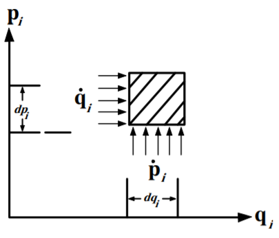
where it is assumed that the infinitessimal volume element \(dv = dq_1, dq_2....dq_s,dp_1, dp_2....dp_s\) contains many possible systems so that \(\rho\) can be considered a continuous distribution. For the conjugate variables \((q_i, p_i)\) shown in Figure \(\PageIndex{1}\), the number of representative points moving across the left-hand edge into the area per unit time is

\[\rho \dot{q}_i dp_i \]

The number of representative points flowing out of the area along the right-hand edge is

\[\left[ \rho \dot{q}_i + \frac{\partial}{ \partial q_i} (\rho \dot{q}_i) dq_i \right] dp_i \]

Hence the net increase in \(\rho\) in the infinitessimal rectangular element \(dq_idp_i\) due to flow in the horizontal direction is

\[− \frac{\partial}{ \partial q_i} (\rho \dot{q}_i) dq_idp_i \]

Similarly, the net gain due to flow in the vertical direction is

\[− \frac{\partial}{ \partial p_i} (\rho \dot{p}_i) dp_idq_i \]

Thus the total increase in the element \(dq_idp_i\) per unit time is therefore

\[− \left[ \frac{\partial}{ \partial q_i } (\rho \dot{q}_i) + \frac{\partial}{ \partial p_i} (\rho \dot{p}_i) \right] dp_idq_i \]

Assume that the total number of points must be conserved, then the total increase in the number of points inside the element \(dq_idp_i\) must equal the net changes in \(\rho\) on the infinitessimal surface element per unit time. That is

\[\left(\frac{\partial \rho}{ \partial t} \right) dq_idp_i \]

Thus summing over all possible values of \(i\) gives

\[\frac{\partial \rho }{\partial t} + \sum_i \left[ \frac{\partial}{ \partial q_i} (\rho \dot{q}_i) + \frac{\partial}{ \partial p_i} (\rho \dot{p}_i) \right] = 0 \]

or

\[\frac{\partial \rho}{ \partial t} +\sum_i \left[ \dot{q}_i \frac{\partial \rho}{ \partial q_i } + \dot{p}_i \frac{\partial \rho}{ \partial p_i} \right] + \rho \sum_i \left[ \frac{\partial \dot{p}_i}{ \partial p_i} + \frac{\partial \dot{q}_i}{ \partial q_i } \right] = 0 \]

Inserting Hamilton’s canonical equations into both brackets and differentiating the last bracket results in

\[\frac{\partial \rho}{ \partial t} +\sum_i \left[ \frac{\partial H}{ \partial p_i} \frac{\partial \rho }{\partial q_i} − \frac{\partial H}{ \partial q_i} \frac{\partial \rho}{ \partial p_i } \right] + \rho \sum_i \left[\frac{ \partial^2 H}{ \partial p_i\partial q_i} − \frac{\partial^2H}{ \partial p_i\partial q_i} \right] = 0 \]

The two terms in the last bracket cancel and thus

\[\frac{\partial \rho }{\partial t} +\sum_i \left[ \frac{\partial H }{\partial p_i} \frac{\partial \rho} { \partial q_i} − \frac{\partial H}{ \partial q_i} \frac{\partial \rho}{ \partial p_i} \right] = \frac{\partial \rho}{ \partial t} + \{\rho , H\} = 0 \]

However, this just equals \(\frac{d\rho}{ dt}\), therefore

\[\frac{d\rho }{dt} = \frac{\partial \rho}{ \partial t} + \{\rho , H\} = 0 \label{15.70}\]

This is called Liouville’s theorem which states that the rate of change of density of representative points vanishes, that is, the density of points is a constant in the Hamiltonian phase space along a specific trajectory. Liouville’s theorem means that the system acts like an incompressible fluid that moves such as to occupy an equal volume in phase space at every instant, even though the shape of the phase-space volume may change, that is, the phase-space density of the fluid remains constant. Equation \ref{15.70} is another illustration of the basic Poisson bracket relation \ref{15.45} and the usefulness of Poisson brackets in physics.

Liouville’s theorem is crucially important to statistical mechanics of ensembles where the exact knowledge of the system is unknown, only statistical averages are known. An example is in focussing of beams of charged particles by beam handling systems. At a focus of the beam, the transverse width in \(x\) is minimized, while the width in \(p_x\) is largest since the beam is converging to the focus, whereas a parallel beam has maximum width \(x\) and minimum spreading width \(p_x\). However, the product \(xp_x\) remains constant throughout the focussing system. For a two dimensional beam, this applies equally for the \(y\) and \(p_y\) coordinates, etc. It is obvious that the final beam quality for any beam transport system is ultimately limited by the emittance of the source of the beam, that is, the initial area of the phase space distribution. Note that Liouville’s theorem only applies to Hamiltonian \(q_i − p_i\) phase space, not to \(x − \dot{x}\) Lagrangian state space. As a consequence, Hamiltonian dynamics, rather than Lagrange dynamics, is used to discuss ensembles in statistical physics.

Note that Liouville’s theorem is applicable only for conservative systems, that is, where Hamilton’s equations of motion apply. For dissipative systems the phase space volume shrinks with time rather than being a constant of the motion.