
19.10: Appendix - Waveform analysis


- Last updated
- Mar 14, 2021
- Save as PDF

( \newcommand{\kernel}{\mathrm{null}\,}\)
Harmonic Waveform Decomposition
Any linear system that is subject to a time-dependent forcing function F(t), can be expressed as a linear superposition of frequency-dependent solutions of the individual harmonic decomposition a(ω) of the forcing function. Similarly, any linear system subject to a spatially-dependent forcing function F(x) can be expressed as a linear superposition of the wavenumber-dependent solutions of the individual harmonic decomposition a(kx) of the forcing function. Fourier analysis provides the mathematical procedure for the transformation between the periodic waveforms and the harmonic content, that is, F(t)⇔a(ω), or F(x)⇔a(kx). Fourier’s theorem states that any arbitrary forcing function F(t) can be decomposed into a sum of harmonic terms. For example for a time-dependent periodic forcing function the decomposition can be a cosine series of the form
F(t)=∞∑n=1αncos(nω0t+ϕn)
where ω0 is the lowest (fundamental) frequency solution. For an aperiodic function a cosine decomposition can be of the form
F(t)=∫∞0α(ω)cos(ωt+ϕ(ω))dω
Either of the complementary functions F(t)⇔a(ω), or F(x)⇔a(kx) are equivalent representations of the harmonic content that can be used to describe signals and waves. The following two sections give an introduction to Fourier analysis.
Periodic systems and the Fourier series
Discrete solutions occur for systems when periodic boundary conditions exist. The response of periodic systems can be described in either the time versus angular frequency domains, or equivalently, the spatial coordinate x versus the corresponding wave number kx. For periodic systems this decomposition leads to the Fourier series where a generalized phase coordinate ϕ can be used to represent either the time or spatial coordinates, that is, with ϕ=ω0t or ϕ=kxx respectively. The Fourier series relates the two representations of the discrete wave solutions for such periodic systems.
Fourier’s theorem states that for a general periodic system any arbitrary forcing function F(ϕ) can be decomposed into a sum of sinusoidal or cosinusoidal terms. The summation can be represented by three equivalent series expansions given below, where ϕ=ω0t or ϕ=k0⋅r, and where ω0,k0 are the fundamental angular frequency and fundamental wave number respectively.
f(ϕ)=a02+∞∑n=1[ancos(nϕ)+bnsin(nϕ)]
f(ϕ)=a02+∞∑n=0cncos(nϕ+φn)
f(ϕ)=a02+∞∑n=0dnsin(nϕ+θn)
where n is an integer, and φn,θn are phase shifts fit to the initial conditions.
The normal modes of a discrete system form a complete set of solutions that satisfy the following orthogonality relation
∫2π0fn(ϕ)fm(ϕ)dϕ=cnδmn
where δmn is the Kronecker delta symbol defined in equation (9.2.10). Orthogonality can be used to determine the coefficients for equations ??? to be
a0=1π∫+π−πf(ϕ)dϕ
an=1π∫+π−πf(ϕ)cos(nϕ)dϕ
bn=1π∫+π−πf(ϕ)sin(nϕ)dϕ
Similarly the coefficients for ??? and ??? are related to the above coefficients by
c2n=d2n=a2n+b2n
Instead of the simple trigonometric form used in equations (??? − ???) the cosine and sine functions can be expanded into the exponential form where
cosϕ=12(eiϕ+e−iϕ)sinϕ=−i2(eiϕ−e−iϕ)
then Equation ??? becomes
f(ϕ)=∞∑n=−∞gneinϕ
where n is any integer and, from the orthogonality, the Fourier coefficients are given by
gn=12π∫+π−πf(ϕ)enϕdϕ
These coefficients are related to the cosine plus sine series amplitudes by
gn=12(an−ibn)
gn=12(an+ibn)
These results show that the coefficients of the exponential series are in general complex, and that they occur in conjugate pairs (that is, the imaginary part of a coefficient an is equal but opposite in sign to that for the coefficient a−n). Although the introduction of complex coefficients may appear unusual, it should be remembered that the real part of a pair of coefficients denotes the magnitude of the cosine wave of the relevant frequency, and that the imaginary part denotes the magnitude of the sine wave. If a particular pair of coefficients an and a−n are real, then the component at the frequency nω0 is simply a cosine; if an and a−n are purely imaginary, the component is just a sine; and if, as is the general case, an and a−n are complex, both cosine and a sine terms are present.
The use of the exponential form of the Fourier series gives rise to the notion of ‘negative frequency’. Of course, f(t)=ancosωnt is a wave of a single frequency ωn=nω0 radians/second, and may be represented by a single line of height an in a normal spectral diagram. However, using the exponential form of the Fourier series results in both positive and negative ω components.
The coexistence of both negative and positive angular frequencies ±ω can be understood by consideration of the Argand diagram where the real component is plotted along the x-axis and the imaginary component along the y-axis. The function gne+iωt represents a vector of length gn that rotates with an angular velocity ω in a positive direction, that is counterclockwise, whereas, gne−iωt represents the vector rotating in a negative direction, that is clockwise. Thus the sum of the two rotating vectors, according to equations ???, leads to cancellation of the opposite components on the imaginary y axis and addition of the two gncosωt real components on the x axis. Subtraction leads to cancellation of the real x components and addition of the imaginary y axis components.
Aperiodic systems and the Fourier Transform
The Fourier transform (also called the Fourier integral) does for the non-repetitive signal waveform what the Fourier series does for the repetitive signal. It was shown that the line spectrum of a recurrent periodic pulse waveform is modified as the pulse duration decreases, assuming the period of the waveform (and hence its fundamental component) remains unchanged. Suppose now that the duration of the pulses remain fixed but the separation between them increases, giving rise to an increasing period. In the limit, only a single rectangular pulse remains, its neighbors having moved away on either side towards ±∞. In this case, the fundamental frequency ω0 tends towards zero and the harmonics become extremely closely spaced and of vanishingly small amplitudes, that is, the system approximates a continuous spectrum.
Mathematically, this situation may be expressed by modifications to the exponential form of the Fourier series already derived. Let the phase factor ϕ=ω0t in Equation ??? then
gn=ω02π∫+π−πf(t)enω0tdt=1τ∫τ2−τ2f(t)enω0tdt
where τ is the period of the periodic force. Let G(ω)=τgn, ω=nω0, and take the limit for τ→∞, then Equation ??? can be written as
G(ω)=∫+∞−∞f(t)eωtdt
Similarly making the same limit for τ→∞ then ω0=2πτ→dω and Equation ??? becomes
f(t)=∞∑n=−∞G(ω)τeinω0t=∞∑n=−∞G(ω)ω02πeiωt=12π∫+∞−∞G(ω)eiωtdω
Equation ??? shows how a non-repetitive time-domain wave form is related to its continuous spectrum. These are known as Fourier integrals or Fourier transforms. They are of central importance for signal processing. For convenience the transforms often are written in the operator formalism using the F symbol in the form
f(t)=12π∫+∞−∞G(ω)eiωtdω≡F−1[12πG(ω)]
G(ω)=∫+∞−∞f(t)e−iωtdt≡Ff(t)
It is very important to grasp the significance of these two equations. The first tells us that the Fourier transform of the waveform f(t) is continuously distributed in the frequency range between ω=±∞, whereas the second shows how, in effect, the waveform may be synthesized from an infinite set of exponential functions of the form e±iωt, each weighted by the relevant value of G(ω). It is crucial to realize that this transformation can go either way equally, that is, from G(ω) to f(t) or vice versa.1
Example 19.10.1: Fourier transform of a single isolated square pulse
Consider a single isolated square pulse of width τ that is described by the rectangular function ∏ defined as
∏(t)={1|t|<τ20|t|>τ2
That is, assume that the amplitude of the pulse is unity between −τ2≤t≤τ2. Then the Fourier transform
G(ω)=∫+τ−τ1.e−iωtdt=τ(sinωτ2ωτ2)
which is an unnormalized sinc(ωτ) function. Note that the width of the pulse Δt=±τ2 leads to a frequency envelope that has the first zeros at Δω=±πτ. Thus the product of these widths Δt⋅Δω=±π which is independent of the width of the pulse, that is Δω=πΔt which is an example of the uncertainty principle which is applicable to all forms of wave motion.
Example 19.10.2: Fourier transform of the Dirac delta function
The Dirac delta function, δ(t−t′), is a pulse of extremely short duration and unit area at t=t′ and is zero at all other times. That is,
1=∫+∞−∞δ(t−t′)dt
The Dirac function, which is sometimes referred to as the impulse function, has many important applications to physics and signal processing. For example, a shell shot from a gun is given a mechanical impulse imparting a certain momentum to the shell in a very short time. Other things being equal, one is interested only in the impulse imparted to the shell, that is, the time integral of the force accelerating the shell in the gun, rather than the details of the time dependence of the force. Since the force acts for a very short time the Dirac delta function can be employed in such problems.
As described in section 3.11 and appendix J, the Dirac delta function is employed in signal processing when signals are sampled for short time intervals. The Fourier transform of the delta function is needed for discussion of sampling of signals
G(ω)=∫+∞−∞δ(t−t′)e−iωtdt=e−iωt′
Since e−iωt essentially is constant over the infinitesimal time duration of the δ(t−t′) function, and the time integral of the δ function is unity, thus the term e−iωt has unit magnitude for any value of ω and has a phase shift of −ω(t−t′) radians. For t′=0 the phase shift is zero and thus the Fourier transform of a Dirac δ(t) function is G(ω)=1. That is, this is a uniform white spectrum for all values of ω.
Time-sampled waveform analysis
An alternative approach for unloosing periodic signals, that is complementary to the Fourier analysis harmonic decomposition, is time-sampled (discrete-sample) waveform analysis where the signal amplitude is measured repetitively at regular time intervals in a time-ordered sequence, that is, a sequence of samples of the instantaneous delta-function amplitudes is recorded. Typically an amplitude-to-digital converter is used to digitize the amplitude for each measured sample and the digital numbers are recorded; this process is called digital signal processing.
The general principles are best explained by first considering the response of a linear system to a step function impulse, followed by a square impulse, and leading to the response of a δ-function impulsive driving force.
Delta-function impulse response
Consider the damped oscillator equation
¨x+Γ˙x+ω20x=F(t)m
and assume that a step function is applied at time t=0. That is;
F(t)m=0t<0F(t)m=at>0
where a is a constant. The initial conditions are that x(0)=˙x(0)=0.
The transient or complementary solution is the solution of the linearly-damped harmonic oscillator
¨x+Γ˙x+ω20x=0
This is independent of the driving force and the solution is given in the chapter 3.5 discussion of the linearly-damped harmonic oscillator.
The particular, steady-state, solution is easy to obtain just by inspection since the force is a constant, that is, the particular solution is
xS=aω20t>0xS=0t<0
Taking the sum of the transient and particular solutions, using the initial conditions, gives the final solution to be
x(t)=aω20[1−e−Γ2tcosω1t−Γe−Γ2t2ω1sinω1t]
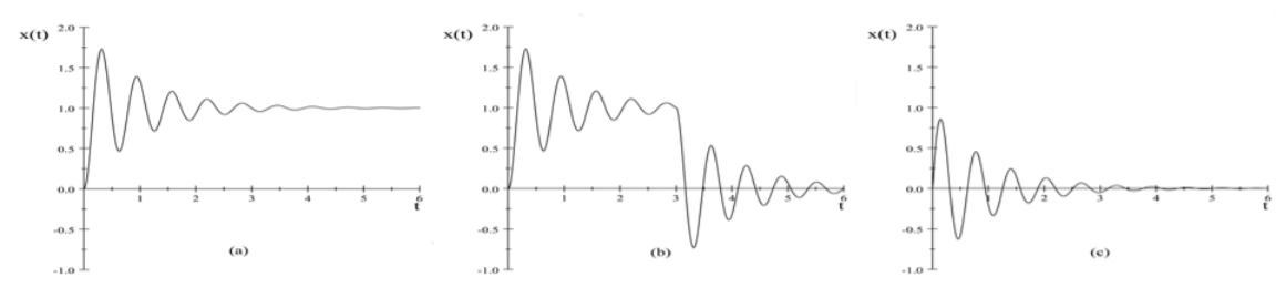
where ω1≡√ω20−(Γ2)2. This functional form is shown in Figure 19.10.1a. Note that the amplitude of the transient response equals −a at t=0 to cancel the particular solution when it jumps to +a. The oscillatory behavior then is just that of the transient response.
A square impulse can be generated by the superposition of two opposite-sign stepfunctions separated by a time τ as shown in Figure 19.10.1b.
The square impulse can be taken to the limit where the width τ is negligibly small relative to the response times of the system. It can be shown that letting τ→0, but keeping the magnitude of the total impulse P=aτ finite for the impulse at time t0, leads to the solution for the δ-function impulse occurring at t0
x(t)=Pω1e−Γ2(t−t0)sinω1(t−t0)t>t0
This response to a delta function impulse is shown in Figure 19.10.1c for the case where t0=0. An example is the response when the hammer strikes a piano string at t=0.
Green’s function waveform decomposition
The response of the linearly-damped linear oscillator to an delta function impulse, that has been expressed above, can be used to exploit the powerful Green’s technique for decomposition of any general forcing function. That is, if the driven system is linear, then the principle of superposition is applicable and allowing expression of the inhomogeneous part of the differential equation as the sum of individual delta functions. That is;
¨x+Γ˙x+ω20x=∞∑n=−∞Fn(t)m=∞∑n=−∞In(t)
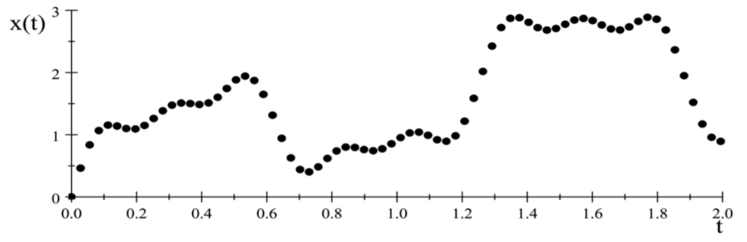
As illustrated in Figure 19.10.2 discrete-time waveform analysis involves repeatedly sampling the instantaneous amplitude in a regular and repetitive sequence of δ-function impulses. Since the superposition principle applies for this linear system then the waveform can be described by a sum of an ordered series of deltafunction impulses where t′ is the time of an impulse. Integrating over all the δ-function responses that have occurred at time t′, that is prior to the time of interest t, leads to
x(t)=∫t−∞F(t′)mω1e−Γ2(t−t′)sinω1(t−t′)dt′t≥t′
The Green’s function G(t−t′) is defined by
G(t−t′)=1mω1e−Γ2(t−t′)sinω1(t−t′)t≥t′=0t<t′
Superposition allows the summed response of the system to be written in an integral form
x(t)=∫t−∞F(t′)G(t−t′)dt′
which gives the final time dependence of the forced system. This repetitive time-sampling approach avoids the need of using Fourier analysis. Note that the Green’s function G(t−t′) includes implicitly the frequency of the free undamped linear oscillator ω0, the free damped linear oscillator ω1≡√ω20−(Γ2)2, as well as the damping coefficient Γ. Access to the combination of fast microcomputers coupled to fast digital sampling techniques has made digital signal sampling the pre-eminent technique for signal recording of audio, video, and detector signal processing.
References
1The only asymmetry in the Fourier transform relations comes from the 2π factor originating from the fact that by convention physicists use the angular frequency ω=2πν rather than the frequency ν. In order to restore symmetry many papers use the factor 1√2π in both relations rather than using the 12π factor in Equation ??? and unity in Equation ???.