12.2: Bernoulli’s Equation

Learning Objectives

By the end of this section, you will be able to:

• Explain the terms in Bernoulli’s equation.
• Explain how Bernoulli’s equation is related to conservation of energy.
• Explain how to derive Bernoulli’s principle from Bernoulli’s equation.
• Calculate with Bernoulli’s principle.
• List some applications of Bernoulli’s principle.

When a fluid flows into a narrower channel, its speed increases. That means its kinetic energy also increases. Where does that change in kinetic energy come from? The increased kinetic energy comes from the net work done on the fluid to push it into the channel and the work done on the fluid by the gravitational force, if the fluid changes vertical position. Recall the work-energy theorem,

\[W_{net} = \dfrac{1}{2} mv^2 - \dfrac{1}{2}mv_0^2.\]

There is a pressure difference when the channel narrows. This pressure difference results in a net force on the fluid: recall that pressure times area equals force. The net work done increases the fluid’s kinetic energy. As a result, the pressure will drop in a rapidly-moving fluid, whether or not the fluid is confined to a tube.

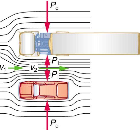
There are a number of common examples of pressure dropping in rapidly-moving fluids. Shower curtains have a disagreeable habit of bulging into the shower stall when the shower is on. The high-velocity stream of water and air creates a region of lower pressure inside the shower, and standard atmospheric pressure on the other side. The pressure difference results in a net force inward pushing the curtain in. You may also have noticed that when passing a truck on the highway, your car tends to veer toward it. The reason is the same—the high velocity of the air between the car and the truck creates a region of lower pressure, and the vehicles are pushed together by greater pressure on the outside (Figure \(\PageIndex{1}\)) This effect was observed as far back as the mid-1800s, when it was found that trains passing in opposite directions tipped precariously toward one another.

Figure \(\PageIndex{1}\): An overhead view of a car passing a truck on a highway. Air passing between the vehicles flows in a narrower channel and must increase its speed (\(v_2\) is greater than \(vv_1\)), causing the pressure between them to drop (\(P_1\) is less than \(P_0\)). Greater pressure on the outside pushes the car and truck together.

Making Connections: Take Home Investigation with a Sheet of Paper:

Hold the short edge of a sheet of paper parallel to your mouth with one hand on each side of your mouth. The page should slant downward over your hands. Blow over the top of the page. Describe what happens and explain the reason for this behavior.

Bernoulli’s Equation

The relationship between pressure and velocity in fluids is described quantitatively by Bernoulli’s equation, named after its discoverer, the Swiss scientist Daniel Bernoulli (1700–1782). Bernoulli’s equation states that for an incompressible, frictionless fluid, the following sum is constant:

\[P + \dfrac{1}{2}\rho v^2 + \rho gh = constant \label{eq1}\]

where \(P\) is the absolute pressure, \(\rho\) is the fluid density, \(v\) is the velocity of the fluid, \(h\) is the height above some reference point, and \(g\) is the acceleration due to gravity. If we follow a small volume of fluid along its path, various quantities in the sum may change, but the total remains constant. Let the subscripts 1 and 2 refer to any two points along the path that the bit of fluid follows; Bernoulli’s equation becomes:

\[P_1 + \underbrace{\dfrac{1}{2}\rho v_1^2}_{\text{kinetic energy}} + \underbrace{\rho gh_1}_{\text{potential energy}} = P_2 + \underbrace{\dfrac{1}{2}\rho v_2^2}_{\text{kinetic energy}} + \underbrace{\rho gh_2. \label{eq2}}_{\text{potential energy}} \]

Bernoulli’s equation is a form of the conservation of energy principle. Note that the second and third terms are the kinetic and potential energy with \(m\) replaced by \(\rho\). In fact, each term in the equation has units of energy per unit volume. We can prove this for the second term by substituting \(\rho = m/V\) into it and gathering terms:

\[\dfrac{1}{2}\rho v^2 = \dfrac{\frac{1}{2}mv^2}{V} = \dfrac{KE}{V}. \label{eq3}\]

So \(\frac{1}{2}\rho v^2\) is the kinetic energy per unit volume. Making the same substitution into the third term of Equation \ref{eq3}, we find

\[\rho gh = \dfrac{mgh}{V} = \dfrac{PE_g}{V}, \label{eq4}\]

so \(\rho gh\) is the gravitational potential energy per unit volume. Note that pressure \(P\) has units of energy per unit volume, too. Since \(P = F/A\), its units are \(N/m^2\). If we multiply these by m/m, we obtain \(N \cdot m/m^3 = J/m^3\), or energy per unit volume. Bernoulli’s equation is, in fact, just a convenient statement of conservation of energy for an incompressible fluid in the absence of friction.

Making Connections: Conservation of Energy

Conservation of energy applied to fluid flow produces Bernoulli’s equation. The net work done by the fluid’s pressure results in changes in the fluid’s \(KE\) and \(PE_g\) per unit volume. If other forms of energy are involved in fluid flow, Bernoulli’s equation can be modified to take these forms into account. Such forms of energy include thermal energy dissipated because of fluid viscosity.

The general form of Bernoulli’s equation has three terms in it (Equation \ref{eq1}), and it is broadly applicable. To understand it better, we will look at a number of specific situations that simplify and illustrate its use and meaning.

Bernoulli’s Equation for Static Fluids

Let us first consider the very simple situation where the fluid is static—that is, \(v_1 = v_2 = 0\). Bernoulli’s equation in that case is

\[P_1 + \rho gh_1 = P_2 + \rho gh_2.\]

We can further simplify the equation by taking \(h_2 = 0\) (we can always choose some height to be zero, just as we often have done for other situations involving the gravitational force, and take all other heights to be relative to this). In that case, we get

\[P_2 = P_1 + \rho gh_1.\]

This equation tells us that, in static fluids, pressure increases with depth. As we go from point 1 to point 2 in the fluid, the depth increases by \(h_1\), and consequently, \(P_2\) is greater than \(P_1\) by an amount \(\rho gh_1\). In the very simplest case, \(P_1\) is zero at the top of the fluid, and we get the familiar relationship \(P = \rho gh\). (Recall that \(P = \rho gh\) and \(\Delta PE_g = mgh\).) Bernoulli’s equation includes the fact that the pressure due to the weight of a fluid is \(\rho gh\). Although we introduce Bernoulli’s equation for fluid flow, it includes much of what we studied for static fluids in the preceding chapter.

Bernoulli’s Principle—Bernoulli’s Equation at Constant Depth

Another important situation is one in which the fluid moves but its depth is constant—that is, \(h_1 = h_2\). Under that condition, Bernoulli’s equation becomes

\[P_1 + \dfrac{1}{2}\rho v_1^2 = P_2 + \dfrac{1}{2}\rho v_2^2.\]

Situations in which fluid flows at a constant depth are so important that this equation is often called Bernoulli’s principle. It is Bernoulli’s equation for fluids at constant depth. (Note again that this applies to a small volume of fluid as we follow it along its path.) As we have just discussed, pressure drops as speed increases in a moving fluid. We can see this from Bernoulli’s principle. For example, if \(v_2\) is greater than \(v_1\) in the equation, then \(P_2\) must be less than \(P_1\) for the equality to hold.

Example \(\PageIndex{1}\): Calculating Pressure: Pressure Drops as a Fluid Speeds Up

Previously, we found that the speed of water in a hose increased from 1.96 m/s to 25.5 m/s going from the hose to the nozzle. Calculate the pressure in the hose, given that the absolute pressure in the nozzle is \(1.01 \times 10^5 \, N/m^2\) (atmospheric, as it must be) and assuming level, frictionless flow.

Strategy

Level flow means constant depth, so Bernoulli’s principle applies. We use the subscript 1 for values in the hose and 2 for those in the nozzle. We are thus asked to find \(P_1\).

Solution

Solving Bernoulli’s principle for \(P_1\) yields

\[\begin{align*} P_1 &= P_2 + \dfrac{1}{2}\rho v_2^2 - \dfrac{1}{2}\rho v_1^2 \\[5pt] &= \dfrac{1}{2}\rho(v_2^2 - v_1^2).\end{align*}\]

Substituting known values,

\[\begin{align*} P_1 &= 1.01 \times 10^5 \, N/m^2 + \dfrac{1}{2}(10^3 \, kg/m^3)[(25.5 m/s)^2 - (1.96 m/s)^2] \\[5pt] &= 4.24 \times 10^5 \, N/m^2.\end{align*}\]

Discussion

This absolute pressure in the hose is greater than in the nozzle, as expected since \(v\) is greater in the nozzle. The pressure \(P_2\) in the nozzle must be atmospheric since it emerges into the atmosphere without other changes in conditions.

Applications of Bernoulli’s Principle

There are a number of devices and situations in which fluid flows at a constant height and, thus, can be analyzed with Bernoulli’s principle.

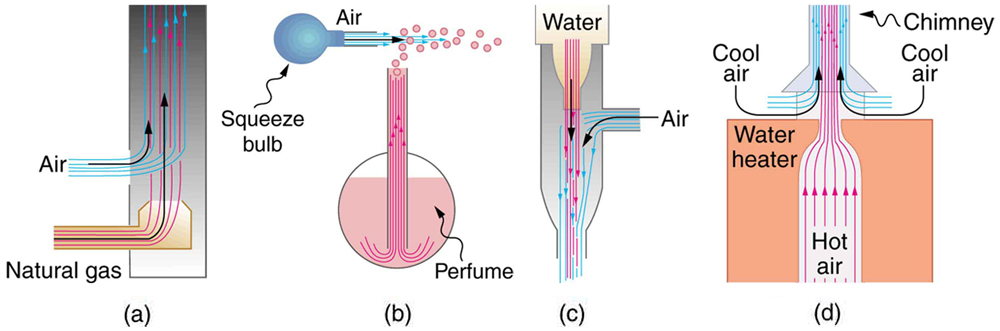
Application: Entrainment

People have long put the Bernoulli principle to work by using reduced pressure in high-velocity fluids to move things about. With a higher pressure on the outside, the high-velocity fluid forces other fluids into the stream. This process is called entrainment. Entrainment devices have been in use since ancient times, particularly as pumps to raise water small heights, as in draining swamps, fields, or other low-lying areas. Some other devices that use the concept of entrainment are shown in Figure \(\PageIndex{2}\).

Figure \(\PageIndex{2}\): Examples of entrainment devices that use increased fluid speed to create low pressures, which then entrain one fluid into another. (a) A Bunsen burner uses an adjustable gas nozzle, entraining air for proper combustion. (b) An atomizer uses a squeeze bulb to create a jet of air that entrains drops of perfume. Paint sprayers and carburetors use very similar techniques to move their respective liquids. (c) A common aspirator uses a high-speed stream of water to create a region of lower pressure. Aspirators may be used as suction pumps in dental and surgical situations or for draining a flooded basement or producing a reduced pressure in a vessel. (d) The chimney of a water heater is designed to entrain air into the pipe leading through the ceiling.

Application: Wings and Sails

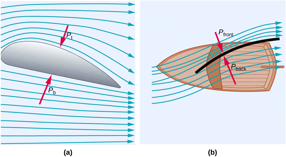
The airplane wing is a beautiful example of Bernoulli’s principle in action. Figure \(\PageIndex{1a}\) shows the characteristic shape of a wing. The wing is tilted upward at a small angle and the upper surface is longer, causing air to flow faster over it. The pressure on top of the wing is therefore reduced, creating a net upward force or lift. (Wings can also gain lift by pushing air downward, utilizing the conservation of momentum principle. The deflected air molecules result in an upward force on the wing — Newton’s third law.) Sails also have the characteristic shape of a wing. (See Figure \(\PageIndex{1b}\).) The pressure on the front side of the sail, \(P_{front}\) is lower than the pressure on the back of the sail, \(P_{back}\). This results in a forward force and even allows you to sail into the wind.

Figure \(\PageIndex{3}\) (a) The Bernoulli principle helps explain lift generated by a wing. (b) Sails use the same technique to generate part of their thrust.

Making Connections: Take Home Investigation with Two Strips of Paper

For a good illustration of Bernoulli’s principle, make two strips of paper, each about 15 cm long and 4 cm wide. Hold the small end of one strip up to your lips and let it drape over your finger. Blow across the paper. What happens? Now hold two strips of paper up to your lips, separated by your fingers. Blow between the strips. What happens?

Application: Velocity Measurement

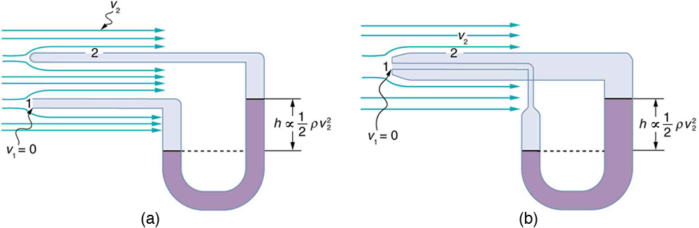
Figure \(\PageIndex{4}\) shows two devices that measure fluid velocity based on Bernoulli’s principle. The manometer in Figure \(\PageIndex{1a}\) is connected to two tubes that are small enough not to appreciably disturb the flow. The tube facing the oncoming fluid creates a dead spot having zero velocity (\(v_1 = 0\)) in front of it, while fluid passing the other tube has velocity \(v_2\). This means that Bernoulli’s principle as stated in

\[P_1 + \dfrac{1}{2}\rho v_1^2 = P_2 + \dfrac{1}{2}\rho v_2^2\]

becomes

\[P_1 = P_2 + \dfrac{1}{2}\rho v_2^2.\]

Thus pressure \(P_2\) over the second opening is reduced by \(\frac{1}{2}\rho v_2^2\), and so the fluid in the manometer rises by \(h\) on the side connected to the second opening, where

\[h \propto \dfrac{1}{2} \rho v_2^2.\]

(Recall that the symbol \(\propto\) means “proportional to.”) Solving for \(v_2\), we see that

\[v_2 \propto \sqrt{h}.\]

Figure \(\PageIndex{1b}\) shows a version of this device that is in common use for measuring various fluid velocities; such devices are frequently used as air speed indicators in aircraft.

Figure \(\PageIndex{4}\): Measurement of fluid speed based on Bernoulli’s principle. (a) A manometer is connected to two tubes that are close together and small enough not to disturb the flow. Tube 1 is open at the end facing the flow. A dead spot having zero speed is created there. Tube 2 has an opening on the side, and so the fluid has a speed \(v\) across the opening; thus, pressure there drops. The difference in pressure at the manometer is \(\frac{1}{2}\rho v_2^2\) and so \(h\) is proportional to \(\frac{1}{2}\rho v_2^2\), (b) This type of velocity measuring device is a Prandtl tube, also known as a pitot tube.

Summary

• Bernoulli’s equation states that the sum on each side of the following equation is constant, or the same at any two points in an incompressible frictionless fluid: \[P_1 + \dfrac{1}{2}\rho v_1^2 + \rho gh_1 = P_2 + \dfrac{1}{2}\rho v_2^2 + \rho gh_2.\]
• Bernoulli’s principle is Bernoulli’s equation applied to situations in which depth is constant. The terms involving depth (or height h ) subtract out, yielding \[P_1 + \dfrac{1}{2}\rho v_1^2 = P_2 + \dfrac{1}{2}\rho v_2^2.\]
• Bernoulli’s principle has many applications, including entrainment, wings and sails, and velocity measurement.

Glossary

Bernoulli’s equation

the equation resulting from applying conservation of energy to an incompressible frictionless fluid: P + 1/2pv² + pgh = constant , through the fluid

Bernoulli’s principle

Bernoulli’s equation applied at constant depth: P₁ + 1/2pv₁² = P₂ + 1/2pv₂²