12.3: The Most General Applications of Bernoulli’s Equation

Learning Objectives

By the end of this section, you will be able to:

• Calculate using Torricelli’s theorem.
• Calculate power in fluid flow.

Torricelli’s Theorem

Figure \(\PageIndex{1}\) shows water gushing from a large tube through a dam. What is its speed as it emerges? Interestingly, if resistance is negligible, the speed is just what it would be if the water fell a distance \(h\) from the surface of the reservoir; the water’s speed is independent of the size of the opening. Let us check this out.

Figure \(\PageIndex{1}\): (a) Jet tubes releasing water in Glen Canyon Dam High Flow Experiment (Bureau of Reclamation): (b) In the absence of significant resistance, water flows from the reservoir with the same speed it would have if it fell the distance \(h\) without friction. This is an example of Torricelli’s theorem.

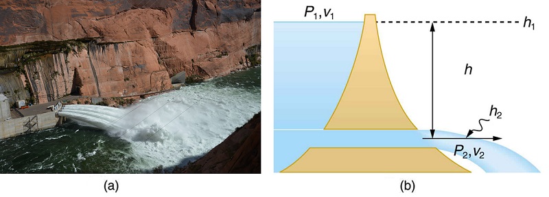
Bernoulli’s equation must be used since the depth is not constant. We consider water flowing from the surface (point 1) to the tube’s outlet (point 2). Bernoulli’s equation as stated in previously is

\[P_1 + \dfrac{1}{2}\rho v_1^2 + \rho gh_1 = P_2 + \dfrac{1}{2}\rho v_2^2 + \rho gh_2.\]

Both \(P_1\) and \(P_2\) equal atmospheric pressure (\(P_1\) is atmospheric pressure because it is the pressure at the top of the reservoir. \(P_2\) must be atmospheric pressure, since the emerging water is surrounded by the atmosphere and cannot have a pressure different from atmospheric pressure.) and subtract out of the equation, leaving

\[\dfrac{1}{2}\rho v_1^2 + \rho gh_1 = \dfrac{1}{2}\rho v_2^2 + \rho gh_2.\]

Solving this equation for \(v_2^2\) noting that the density \(\rho\) cancels (because the fluid is incompressible), yields

\[v_2^2 = v_1^2 + 2g(h_1 - h_2).\]

We let \(h = h_1 - h_2\), the equation then becomes

\[v_2^2 = v_1^2 + 2gh\]

where \(h\) is the height dropped by the water. This is simply a kinematic equation for any object falling a distance \(h\) with negligible resistance. In fluids, this last equation is called Torricelli’s theorem. Note that the result is independent of the velocity’s direction, just as we found when applying conservation of energy to falling objects.

Figure \(\PageIndex{2}\): Pressure in the nozzle of this fire hose is less than at ground level for two reasons: the water has to go uphill to get to the nozzle, and speed increases in the nozzle. In spite of its lowered pressure, the water can exert a large force on anything it strikes, by virtue of its kinetic energy. Pressure in the water stream becomes equal to atmospheric pressure once it emerges into the air.

All preceding applications of Bernoulli’s equation involved simplifying conditions, such as constant height or constant pressure. The next example is a more general application of Bernoulli’s equation in which pressure, velocity, and height all change. (See Figure.)

Example \(\PageIndex{1}\): Calculating Pressure: A Fire Hose Nozzle

Fire hoses used in major structure fires have inside diameters of 6.40 cm. Suppose such a hose carries a flow of 40.0 L/s starting at a gauge pressure of \( 1.62 \times 10^6 \, N/m^2\). The hose goes 10.0 m up a ladder to a nozzle having an inside diameter of 3.00 cm. Assuming negligible resistance, what is the pressure in the nozzle?

Strategy

Here we must use Bernoulli’s equation to solve for the pressure, since depth is not constant.

Solution

Bernoulli’s equation states

\[P_1 + \dfrac{1}{2}\rho v_1^2 + \rho gh_1 = P_2 + \dfrac{1}{2}\rho v_2^2 + \rho gh_2,\nonumber\]

where the subscripts 1 and 2 refer to the initial conditions at ground level and the final conditions inside the nozzle, respectively. We must first find the speeds \(v_1\) and \(v_2\). Since \(Q = A_1v_1\), we get

\[\begin{align*}v_1 &= \dfrac{Q}{A_1} \\[5pt] &= \dfrac{40.0 \times 10^{-3} m^3/s}{\pi(3.20 \times 10^{-2} m)^2} \\[5pt] &= 12.4 \, m/s. \end{align*}\]

Similarly, we find

\[v_2 = 56.6 \, m/s.\nonumber\]

(This rather large speed is helpful in reaching the fire.) Now, taking \(h_1\) to be zero, we solve Bernoulli’s equation for \(P_2\):

\[P_2 = P_1 + \dfrac{1}{2}\rho(v_1^2 - v_2^2) - \rho gh_2. \nonumber\]

Substituting known values yields

\[\begin{align*} P_2 &= 1.62 \times 10^6 N/m^2 + \dfrac{1}{2}(1000 \, kg/m^3)[(12.4 \, m/s)^2 - (56.6 \, m/s)^2] - (1000 \, kg/m^3)(9.80 m/s^2)(10.0 \, m) \\[5pt] &= 0 \end{align*}\]

Discussion

This value is a gauge pressure, since the initial pressure was given as a gauge pressure. Thus the nozzle pressure equals atmospheric pressure, as it must because the water exits into the atmosphere without changes in its conditions.

Power in Fluid Flow

Power is the rate at which work is done or energy in any form is used or supplied. To see the relationship of power to fluid flow, consider Bernoulli’s equation:

\[P + \dfrac{1}{2}\rho v^2 + \rho gh = constant.\]

All three terms have units of energy per unit volume, as discussed in the previous section. Now, considering units, if we multiply energy per unit volume by flow rate (volume per unit time), we get units of power. That is \((E/V)(V/t) = E/t\). This means that if we multiply Bernoulli’s equation by flow rate \(Q\), we get power. In equation form, this is

\[\left(P + \dfrac{1}{2}\rho v^2 + \rho gh \right)Q = power.\]

Each term has a clear physical meaning. For example, \(PQ\) is the power supplied to a fluid, perhaps by a pump, to give it its pressure \(P\). Similarly, \(\frac{1}{2}\rho v^2Q\) is the power supplied to a fluid to give it its kinetic energy. And \(\rho ghQ\) is the power going to gravitational potential energy.

Making Connections: Power

Power is defined as the rate of energy transferred, or \(E/t\). Fluid flow involves several types of power. Each type of power is identified with a specific type of energy being expended or changed in form.

Example \(\PageIndex{2}\): Calculating Power in a Moving Fluid

Suppose the fire hose in the previous example is fed by a pump that receives water through a hose with a 6.40-cm diameter coming from a hydrant with a pressure of \(0.700 \times 10^6 \, N/m^2\). What power does the pump supply to the water?

Strategy

Here we must consider energy forms as well as how they relate to fluid flow. Since the input and output hoses have the same diameters and are at the same height, the pump does not change the speed of the water nor its height, and so the water’s kinetic energy and gravitational potential energy are unchanged. That means the pump only supplies power to increase water pressure by \(0.92 \times 10^6 \, N/m^2\) (from \(0.700 \times 10^6 \, N/m^2 \) to \(1.62 \times 10^6 \, N/m^2)\).

Solution

As discussed above, the power associated with pressure is

\[\begin{align*} power &= PQ \\[5pt] &= (0.920 \times 10^6 \, N/m^2)(40.0 \times 10^{-3} m^3/s).\\[5pt] &= 3.68 \times 10^4 \, W \\[5pt] &= 36.8 \, kW \end{align*} \]

Discussion

Such a substantial amount of power requires a large pump, such as is found on some fire trucks. (This kilowatt value converts to about 50 hp.) The pump in this example increases only the water’s pressure. If a pump—such as the heart—directly increases velocity and height as well as pressure, we would have to calculate all three terms to find the power it supplies.

Summary

• Power in fluid flow is given by the equation \((P_1 + \frac{1}{2}\rho v^2 + \rho gh)Q = power\), where the first term is power associated with pressure, the second is power associated with velocity, and the third is power associated with height.