
22.8: Torque on a Current Loop - Motors and Meters
- Page ID
- 2702

Learning Objectives
By the end of this section, you will be able to:
- Describe how motors and meters work in terms of torque on a current loop.
- Calculate the torque on a current-carrying loop in a magnetic field.
Motors are the most common application of magnetic force on current-carrying wires. Motors have loops of wire in a magnetic field. When current is passed through the loops, the magnetic field exerts torque on the loops, which rotates a shaft. Electrical energy is converted to mechanical work in the process (Figure \(\PageIndex{1}\)).
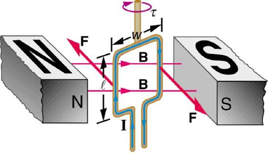
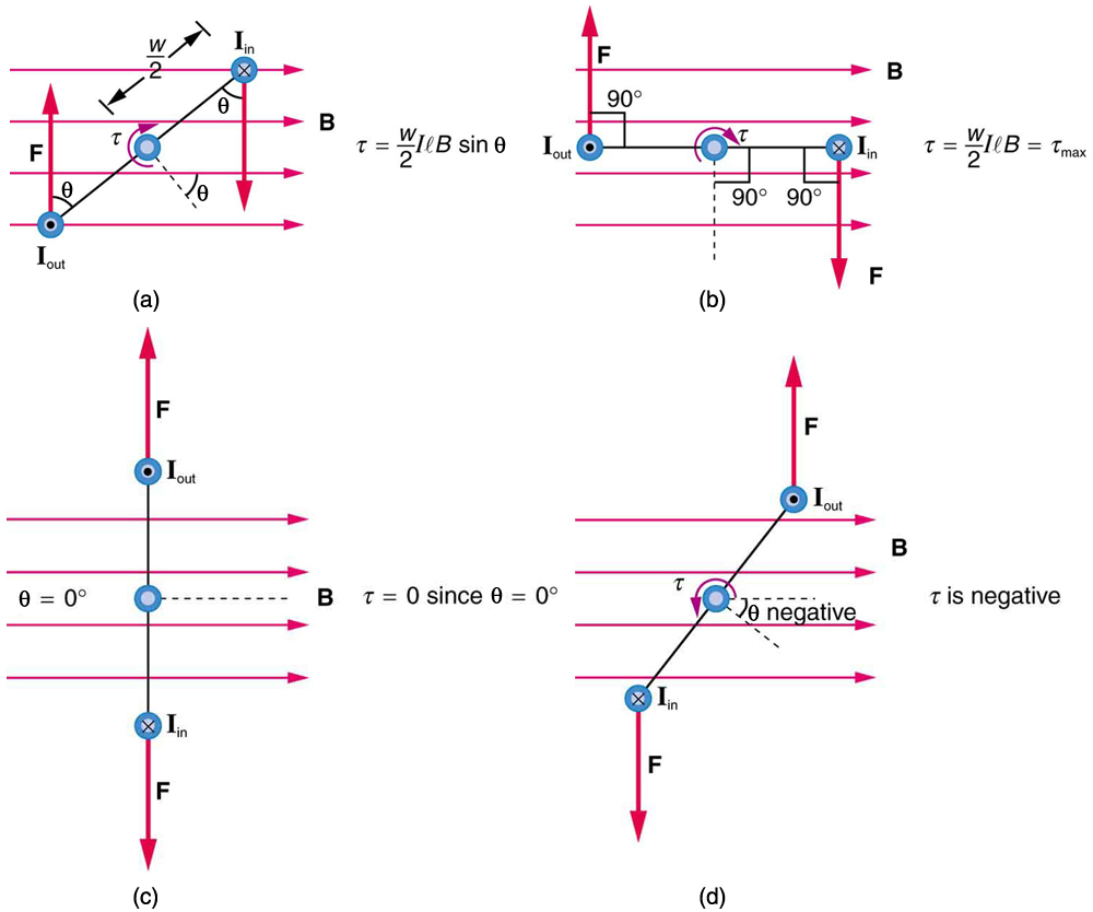
Let us examine the force on each segment of the loop in Figure 1 to find the torques produced about the axis of the vertical shaft. (This will lead to a useful equation for the torque on the loop.) We take the magnetic field to be uniform over the rectangular loop, which has width \(w\) and height \(l\). First, we note that the forces on the top and bottom segments are vertical and, therefore, parallel to the shaft, producing no torque. Those vertical forces are equal in magnitude and opposite in direction, so that they also produce no net force on the loop. Figure \(\PageIndex{2}\) shows views of the loop from above. Torque is defined as \(\tau = rF\sin \theta \), where \(F\) is the force, \(r\) is the distance from the pivot that the force is applied, and \(\theta\) is the angle between \(r\) and \(F\). As seen in Figure \(\PageIndex{1a}\), right hand rule 1 gives the forces on the sides to be equal in magnitude and opposite in direction, so that the net force is again zero. However, each force produces a clockwise torque. Since \(r = w/2\), the torque on each vertical segment is \(\left( w/2\right)F\sin\theta\), and the two add to give a total torque
\[\tau = \frac{w}{2}F\sin\theta + \frac{2}{2}F\sin\theta = wF\sin\theta \label{22.9.1}\]
Now, each vertical segment has a length \(l\) that is perpendicular to \(B\), so that the force on each is \(F = \pi B\). Entering \(F\) into the expression for torque yields
\[\tau = w \pi B \sin \theta.\label{22.9.2}\]
If we have a multiple loop of \(N\) turns, we get \(N\) times the torque of one loop. Finally, note that the area of the loop is \(A = wl\); the expression for the torque becomes
\[\tau = NIAB \sin \theta.\label{22.9.3}\]
This is the torque on a current-carrying loop in a uniform magnetic field. This equation can be shown to be valid for a loop of any shape. The loop carries a current \(I\), has \(N\) turns, each of area \(A\), and the perpendicular to the loop makes an angle \(\theta\) with the field \(B\). The net force on the loop is zero.
Example \(\PageIndex{1}\): Calculating Torque on a Current-Carrying Loop in a Strong Magnetic Field
Find the maximum torque on a 100-turn square loop of a wire of 10.0 cm on a side that carries 15.0 A of current in a 2.00-T field.
Strategy
Torque on the loop can be found using \(\tau = NIAB\sin\theta\). Maximum torque occurs when \(\theta = 90^{\circ}\) and \(\sin \theta = 1\).
Solution
For \(\sin \theta = 1\), the maximum torque is
\[\tau_{max} = NIAB.\nonumber\]
Entering known values yields
\[ \begin{align*} \tau_{max} &= \left(100\right)\left(15.0 A\right)\left(0.100 m^{2}\left)\right(2.00 T\right) \\[5pt] &= 30.0 N \cdot m. \end{align*}\]
Discussion
This torque is large enough to be useful in a motor.
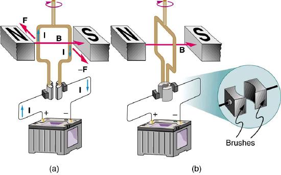
The torque found in the preceding example is the maximum. As the coil rotates, the torque decreases to zero at \(\theta = 0\). The torque then reverses its direction once the coil rotates past \(\theta = 0\) (Figure \(\PageIndex{1d}\)). This means that, unless we do something, the coil will oscillate back and forth about equilibrium at \(\theta = 0\). This means that, unless we do something, the coil will oscillate back and forth about equilibrium at \(\theta = 0\) with automatic switches called brushes (Figure \(\PageIndex{3}\)).
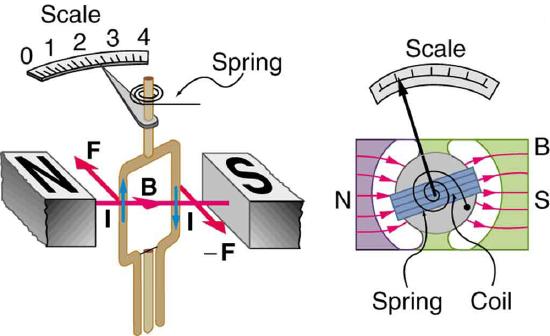
Meters, such as those in analog fuel gauges on a car, are another common application of magnetic torque on a current-carrying loop. Figure \(\PageIndex{4}\) shows that a meter is very similar in construction to a motor. The meter in the figure has its magnets shaped to limit the effect of \(\theta\) by making \(B\) perpendicular to the loop over a large angular range. Thus the torque is proportional to \(I\) and not \(\theta\). A linear spring exerts a counter-torque that balances the current-produced torque. This makes the needle deflection proportional to \(I\). If an exact proportionality cannot be achieved, the gauge reading can be calibrated. To produce a galvanometer for use in analog voltmeters and ammeters that have a low resistance and respond to small currents, we use a large loop area \(A\), high magnetic field \(B\), and low-resistance coils.
Summary
- The torque \(\tau\) on a current-carrying loop of any shape in a uniform magnetic field. is \[\tau = NIAB\sin\theta, \nonumber\] where \(N\) is the number of turns, \(I\) is the current, \(A\) is the area of the loop, \(B\) is the magnetic field strength, and \(\theta\) is the angle between the perpendicular to the loop and the magnetic field.
Glossary
- motor
- loop of wire in a magnetic field; when current is passed through the loops, the magnetic field exerts torque on the loops, which rotates a shaft; electrical energy is converted to mechanical work in the process
- meter
- common application of magnetic torque on a current-carrying loop that is very similar in construction to a motor; by design, the torque is proportional to \(I\) and not, so the needle deflection is proportional to the current