4.1: Introduction to Vectors

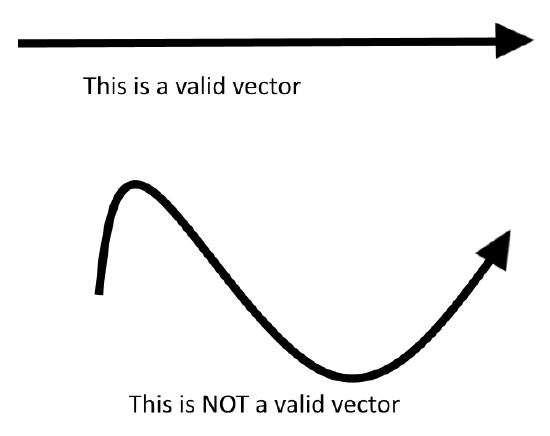
As we have discussed before, a vector is just a scalar pointing in a specific direction. It is represented by an arrow of length equal to its magnitude and pointing in the direction of the vector. The "line part"/"scalar part" of the vector is called its tail and the "direction part"/tip is called the head. Keep in mind that a vector arrow is completely straight and never curved.

 

 

 

 

 

 

 

 

 

 

By convention, vectors are either denoted by a little arrow on top of the character (\(\overrightarrow{a} or \overrightarrow{AB}\)) or as a bold character (a or AB). Though the basic idea of a vector is quite simple, using it correctly can simplify your problems a lot. For example, in the case of rotating bodies, instead of dealing with the huge number of various linear speeds, we simply take a vector (rather, a pseudovector) along its axis of rotation. This application will be discussed in the chapter 'Uniform Circular Motion.'

In this book, we shall restrict our discussion to Cartesian vectors, i.e. vectors on the Cartesian plane.

 

Comparing vectors

Two vectors are said to be equal to each other if they point in the same direction and have the same length.

In mathematical terms, vectors that have the same magnitude (length) and make the same angles with corresponding axes (direction), they are said to be equal. Or an another way to say this is that if two vectors can be superimposed/overlayed on each other such that they cover each other perfectly, they are equal.

Note that the position of the vector in space does not matter, just the direction and magnitude. This is because unless it's a position vector, where it is located does not matter.

If representing the vector as a matrix or a sum of unit vectors (discussed below), if the matrix or unit vector sum of two vectors is equal, they are said to be equal.

 

Addition & Subtraction of vectors

Adding vectors is basically walking along the path the vectors lay out for you. The resultant vector is the vector pointing from your initial position to your final position. This "walking along" method is referred to as the triangle method of vector addition. Every vector addition method is the triangle method in another form. Subtracting vectors is the exact same as adding them, except you have to invert/flip the direction of the vector being subtracted/"removed". Here, we shall discuss 2 methods of addition/subtraction.

Method 1: Triangle method

As discussed above, the triangle method is the most basic method. The walking analogy is useful to remember, as it prevents any confusion about the placement of the vectors while using this method. The process is as follows:

1. Place the vectors so as to create the walking path. This is done by placing the head of the first vector onto the tail of the second. Remember that though we can "slide" the vectors around our space, we cannot rotate the vectors.
2. For subtracting a vector, simply rotate it 180^o.
3. Repeat steps 1 and 2 until we have used up all of the vectors we wish to add together.
4. Draw a vector from the tail of the first vector to the head of the last. This vector we just drew is our resultant vector.

This process is demonstrated in this GIF:

This same method can be applied in 3D, 4D and beyond. But as you can imagine, that would be very hard to do, owing the the lack of 3D or 4D graph paper. Furthermore, this method can be quite time-consuming and inaccurate because we have to hand-drawn or assemble these vectors and lay them out. So, we shall convert this whole method into a mathematical equation.

Method 2: Parallelogram method

Recall from middle-school geometry that a parallelogram consists of two congruent triangles. In other words, the parallel sides of a parallelogram can be described as equal vectors. So, the vector addition can be represented as shown:

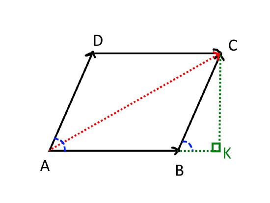
Keep in mind that the angle between two vectors is measured by connecting their tails.

In this figure, the important things to note are as follows:

1. In \(\Delta ABC\) we have used the triangle method for vector addition
2. As \(AC\) is a diagonal of a parallelogram, \(\Delta CDA\) and \(\Delta ABC\) are congruent
3. We have constructed an altitude \(CK\)
4. \(\angle CBK = \angle DAB \) because corresponding angles of a transversal of two parallel lines are equal. Lets call that angle \(\theta\)

We can conclude that \(\overrightarrow{BC} = \overrightarrow{AD}\)    ....(i)     ∵ Congruency

Also, by the Pythagoras theorem, \( (AC)^2 = (CK)^2 + (AK)^2 \)    ....(ii)

But \((AK) = (AB) + (BK) \), and \((BK) = (BC)\cos\theta\)

And \((CK) = (BC)\sin\theta \)

∴ \((AC)^2 = (AB)^2 + (BC)^2 \cos^2 \theta + 2(BC)\cos \theta + (BC)^2 \sin^2 \theta \)    ....(iii)

Using (i) and \(\sin^2 x + \cos^2 x = 1 \) in (iii),

\[(AC)^2 = (AB)^2 + (AD)^2 + 2(AB)(AD)\cos \theta \nonumber \]

Remember this equation. However, note that this equation only gives us the magnitude of the resultant vector. To get the angle between \(\overrightarrow{AB} \) and \(\overrightarrow{AC} \), we use the following formula:

\[\tan \alpha = \dfrac{(AD)\sin \theta}{(AB) + (AD)\cos \theta} \nonumber \]

Where \(\alpha\) is the required angle. The derivation of this formula is quite simple and is left as an exercise to the reader (HINT: Use \(\cos \theta = \dfrac{(BK)}{(BC)} \))