
11.3: Production and Properties of Electromagnetic Waves


( \newcommand{\kernel}{\mathrm{null}\,}\)
Learning Objectives
- Describe the electric and magnetic waves as they move out from a source, such as an AC generator.
- Describe the momentum carried by electromagnetic waves and its relationship to radiation pressure.
We can get a good understanding of electromagnetic waves (EM) by considering how they are produced. Whenever a current varies, associated electric and magnetic fields vary, moving out from the source like waves. Perhaps the easiest situation to visualize is a varying current in a long straight wire, produced by an AC generator at its center, as illustrated in Figure 11.3.1.
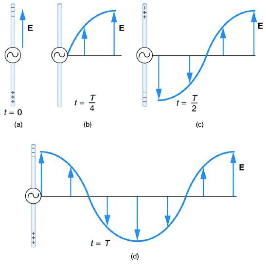
The electric field (E) shown surrounding the wire is produced by the charge distribution on the wire. Both the E and the charge distribution vary as the current changes. The changing field propagates outward at the speed of light.
There is an associated magnetic field (B) which propagates outward as well (see Figure 11.3.2). The electric and magnetic fields are closely related and propagate as an electromagnetic wave. This is what happens in broadcast antennae such as those in radio and TV stations.
Closer examination of the one complete cycle shown in Figure 11.3.1 reveals the periodic nature of the generator-driven charges oscillating up and down in the antenna and the electric field produced. At time t=0, there is the maximum separation of charge, with negative charges at the top and positive charges at the bottom, producing the maximum magnitude of the electric field (or E-field) in the upward direction. One-fourth of a cycle later, there is no charge separation and the field next to the antenna is zero, while the maximum E-field has moved away at speed c.
As the process continues, the charge separation reverses and the field reaches its maximum downward value, returns to zero, and rises to its maximum upward value at the end of one complete cycle. The outgoing wave has an amplitude proportional to the maximum separation of charge. Its wavelength (λ) is proportional to the period of the oscillation and, hence, is smaller for short periods or high frequencies. (As usual, wavelength and frequency (f) are inversely proportional.)
Electric and Magnetic Waves: Moving Together
Following Ampere’s law, current in the antenna produces a magnetic field, as shown in Figure 11.3.2. The relationship between E and B is shown at one instant in Figure 11.3.2(a). As the current varies, the magnetic field varies in magnitude and direction.
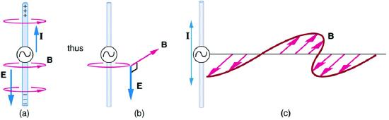
The magnetic field lines also propagate away from the antenna at the speed of light, forming the other part of the electromagnetic wave, as seen in Figure 11.3.2(b). The magnetic part of the wave has the same period and wavelength as the electric part, since they are both produced by the same movement and separation of charges in the antenna.
The electric and magnetic waves are shown together at one instant in time in Figure 11.3.3. The electric and magnetic fields produced by a long straight wire antenna are exactly in phase. Note that they are perpendicular to one another and to the direction of propagation, making this a transverse wave.
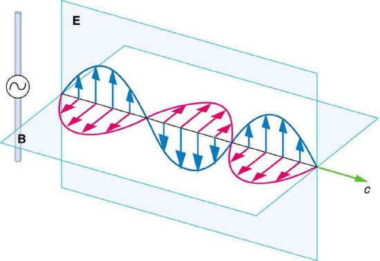
Electromagnetic waves generally propagate out from a source in all directions, sometimes forming a complex radiation pattern. A linear antenna like this one will not radiate parallel to its length, for example. The wave is shown in one direction from the antenna in Figure 11.3.3 to illustrate its basic characteristics.
Instead of the AC generator, the antenna can also be driven by an AC circuit. In fact, charges radiate whenever they are accelerated. But while a current in a circuit needs a complete path, an antenna has a varying charge distribution forming a standing wave, driven by the AC. The dimensions of the antenna are critical for determining the frequency of the radiated electromagnetic waves. This is a resonant phenomenon and when we tune radios or TV, we vary electrical properties to achieve appropriate resonant conditions in the antenna.
Receiving Electromagnetic Waves
Electromagnetic waves carry energy away from their source, similar to a sound wave carrying energy away from a standing wave on a guitar string. An antenna for receiving EM signals works in reverse. And like antennas that produce EM waves, receiver antennas are specially designed to resonate at particular frequencies.
An incoming electromagnetic wave accelerates electrons in the antenna, setting up a standing wave. If the radio or TV is switched on, electrical components pick up and amplify the signal formed by the accelerating electrons. The signal is then converted to audio and/or video format. Sometimes big receiver dishes are used to focus the signal onto an antenna.
In fact, charges radiate whenever they are accelerated. When designing circuits, we often assume that energy does not quickly escape AC circuits, and mostly this is true. A broadcast antenna is specially designed to enhance the rate of electromagnetic radiation, and shielding is necessary to keep the radiation close to zero. Some familiar phenomena are based on the production of electromagnetic waves by varying currents. Your microwave oven, for example, sends electromagnetic waves, called microwaves, from a concealed antenna that has an oscillating current imposed on it.
Momentum Carried by Electromagnetic Waves
As electromagnetic waves are received, as described above, the forces exerted on the charged particles (see [link]1 for diagrams) do work on the particles and increase its energy. The energy that sunlight carries is a familiar part of every warm sunny day. A much less familiar feature of electromagnetic radiation is the extremely weak pressure that electromagnetic radiation produces by exerting a force in the direction of the wave. This force occurs because electromagnetic waves contain and transport momentum.
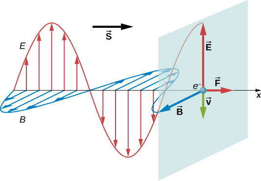
To understand the direction of the force for a very specific case, consider a plane electromagnetic wave incident on a metal. The electrons in the metal move with the velocity v that is proportional to the force on it due to applied electric force (in opposite direction to E because electron is negatively charged). There are other, frictional forces in the metal that make this motion happen (this is the origin of Ohm's law in electric circuits). Note that there is also a magnetic field in the electromagnetic wave (Figure 11.3.4). Using the right-hand rule (magnetic force is F=q(v×B)), we can get the direction of force on the electron (remember that electron is negatively charged), which is shown in Figure 11.3.4. This force is in the same direction as the direction of wave propagation, and it represents a transfer of momentum carried by the electromagnetic wave from the wave to the electron. This momentum is directly proportional to the energy carried by the electromagnetic wave and is given by,
p=Ec,
where p is the magnitude of momentum of electromagnetic wave, E is the energy of electromagnetic wave, and c is the speed of light.
Maxwell predicted that an electromagnetic wave carries momentum. An object absorbing an electromagnetic wave would experience a force in the direction of propagation of the wave. The force corresponds to radiation pressure exerted on the object by the wave. The force would be twice as great if the radiation were reflected rather than absorbed, because the change in the momentum of electromagnetic wave itself is twice as great (and we enforce momentum conservation of the system as a whole).
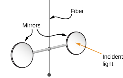
Maxwell’s prediction was confirmed in 1903 by Nichols and Hull by precisely measuring radiation pressures with a torsion balance. The schematic arrangement is shown in Figure 11.3.5. The mirrors suspended from a fiber were housed inside a glass container. Nichols and Hull were able to obtain a small measurable deflection of the mirrors from shining light on one of them. From the measured deflection, they could calculate the unbalanced force on the mirror, and obtained agreement with the predicted value of the force.
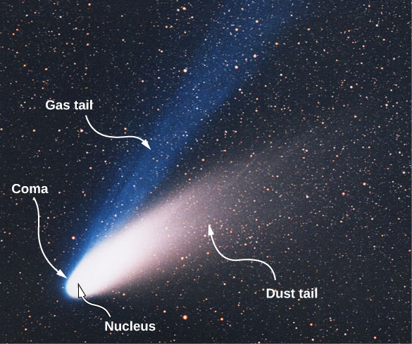
Radiation pressure plays a role in explaining many observed astronomical phenomena, including the appearance of comets. Comets are basically chunks of icy material in which frozen gases and particles of rock and dust are embedded. When a comet approaches the Sun, it warms up and its surface begins to evaporate. The coma of the comet is the hazy area around it from the gases and dust. Some of the gases and dust form tails when they leave the comet. Notice in Figure 11.3.6 that a comet has two tails. The ion tail (or gas tail in Figure 11.3.6) is composed mainly of ionized gases. These ions interact electromagnetically with the solar wind, which is a continuous stream of charged particles emitted by the Sun. The force of the solar wind on the ionized gases is strong enough that the ion tail almost always points directly away from the Sun. The second tail is composed of dust particles. Because the dust tail is electrically neutral, it does not interact with the solar wind. However, this tail is affected by the radiation pressure produced by the light from the Sun. Although quite small, this pressure is strong enough to cause the dust tail to be displaced from the path of the comet.
After Maxwell showed that light carried momentum as well as energy, a novel idea eventually emerged, initially only as science fiction. Perhaps a spacecraft with a large reflecting solar sail could use radiation pressure for propulsion. Such a vehicle would not have to carry fuel. It would experience a constant but small force from solar radiation, instead of the short bursts from rocket propulsion. It would accelerate slowly, but by being accelerated continuously, it would eventually reach great speeds. A spacecraft with small total mass and a sail with a large area would be necessary to obtain a usable acceleration.
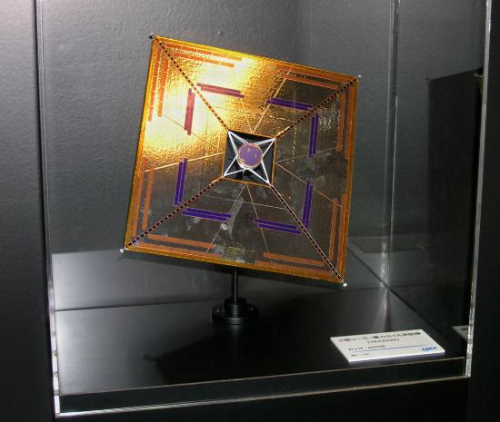
The latest accomplishment on this concept is represented by the IKAROS (Interplanetary Kite-craft Accelerated by Radiation Of the Sun) project by Japan Aerospace Exploration Agency (JAXA), which was launched in May 2010. IKAROS solar sail is currently traveling through the solar system. During its six-month journey to Venus, acceleration and attitude control using the solar sail, rather than thrusters, were successfully tested. Last update from the spacecraft was in May 2014, on a ten-month orbit around the Sun. A scale model of the spacecraft is shown in Figure 11.3.7.
Section Summary
- Electromagnetic waves are created by oscillating charges (which radiate whenever accelerated) and have the same frequency as the oscillation.
- Since the electric and magnetic fields in most electromagnetic waves are perpendicular to the direction in which the wave moves, it is ordinarily a transverse wave.
- Electromagnetic waves carry momentum and exert radiation pressure.
- The momentum of an electromagnetic wave is directly proportional to its energy.
Glossary
- electric field
- a vector quantity (E); the lines of electric force per unit charge, moving radially outward from a positive charge and in toward a negative charge
- electric field strength
- the magnitude of the electric field, denoted E-field
- magnetic field
- a vector quantity (B); can be used to determine the magnetic force on a moving charged particle
- magnetic field strength
- the magnitude of the magnetic field, denoted B-field
- transverse wave
- a wave, such as an electromagnetic wave, which oscillates perpendicular to the axis along the line of travel
- standing wave
- a wave that oscillates in place, with nodes where no motion happens
- wavelength
- the distance from one peak to the next in a wave
- amplitude
- the height, or magnitude, of an electromagnetic wave
- frequency
- the number of complete wave cycles (up-down-up) passing a given point within one second (cycles/second)
- resonant
- a system that displays enhanced oscillation when subjected to a periodic disturbance of the same frequency as its natural frequency
- oscillate
- to fluctuate back and forth in a steady beat
- radiation pressure
- pressure exerted by an electromagnetic wave on a surface
- solar sail
- a spacecraft that utilizes radiation pressure due to solar radiation in its propulsion
1 Section 16.2: Maxwell’s Equations and Electromagnetic Waves
University Physics II - Thermodynamics, Electricity, and Magnetism