5.6: Forces on Magnetic Circuits


- Last updated
- Jun 21, 2021
- Save as PDF

( \newcommand{\kernel}{\mathrm{null}\,}\)
The induction coefficients, Equation (5.5.2), are functions of coil position and coil geometry. If a circuit is moved, or if its shape is altered, the fluxes through all the circuits will be altered. A changing magnetic flux through a circuit induces an emf in that circuit:
curl(E)=−∂→B∂t,
so that
∫∫Surfacecurl(→E)⋅d→S=−∫∫Surface∂→B∂t⋅d→S=−∂∂t∫∫Surface→B⋅d→S.
But the last term above is just the time rate of change of the magnetic flux, therefore
∫∫Surfacecurl(→E)⋅d→S=−dΦdt.
Stokes’ theorem can be used to transform the surface integral of curl(→E) over the area of a circuit into a line integral of the electric field around the circuit contour C:
e=∮C→E⋅d→L=−dΦdt.
In order to be able to use conservation of energy to derive formulae that relate the forces exerted by the magnetic field on circuits to the change in magnetic energy that accompanies any shift in position or distortion in shape of those circuits, it is useful to consider wires that are made of perfectly superconducting metals so that resistive losses can be neglected. Magnetic forces can not depend upon the circuit resistances because these forces depend only upon the interaction between a current element and the magnetic field acting upon that current element. The emf around a closed superconducting loop must be zero because the electric field in a perfect conductor must always be zero; any electric field strength would produce an infinite current. It follows that the fluxes through closed superconducting circuits cannot change. Any relative motion of the circuits, or any distortion of the circuits, must be accompanied by changes in their currents such that the fluxes remain constant. In addition, energy must be conserved, and therefore any external work done by the magnetic forces during a displacement must be at the expense of the magnetic energy stored in the system
→FM⋅δ→r=−δUB.
The magnetic energy acts like a potential energy function for the magnetic forces.
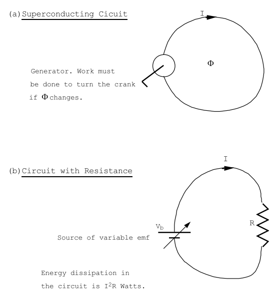
Usually it is convenient to arrange to keep the current in each circuit constant during the circuit motion or deformation. The current can be kept constant, in principle, by including a superconducting generator in each circuit as is shown in Figure (5.6.9(a)). This is a device by means of which external electrical work can be done on the circuit. Now the flux through the circuit can be allowed to change because the electromotive force (emf) due to the changing flux can be cancelled out by the external emf of the generator so that the net emf in the system can be maintained at zero. In order to cancel out the emf due to the changing flux, work must be done on the generator at the rate
dWdt=egenI=−eI=IdΦdt,
or the change in flux, dΦ, must be accompanied by an input of external work (to turn the crank on the generator) such that
dW=IdΦ.
A similar argument can be applied to each circuit of N coupled circuits so that taken all together the total external energy input through the generators is
dW=N∑n=1INdΦN.
As mentioned above, the result (???) cannot depend upon whether or not the circuits contain resistance elements. A circuit that contains a resistance must be provided with a source of emf in order to maintain a constant current (see Figure (5.6.9(b)). This emf, that can be imagined to be a power supply whose terminal voltage is variable, must supply energy at the rate of I2R Watts, where R is the circuit resistance. If the flux through the circuit increases the power supply voltage must be increased by e = dΦ/dt in order to maintain the current constant. This means that the power extracted from the power supply must also increase by the amount
dWdt=eI=IdΦdt.
In order to change the flux through the circuit by dΦ at fixed current the power supply must add extra energy in the amount
dW=IdΦ,
and this clearly does not depend upon whether there is, or is not, resistance in the circuit. A generalization of this result to a collection of N circuits leads directly to Equation (???). Any displacement of a circuit, or a deformation of a circuit, that results in a change of the inductance coefficients must result in a change in the magnetic energy stored in the field if the current in each of the circuits is held fixed. This energy change is given by
dUB=12∑NINdΦN,
see Equation (5.4.9). But in view of Equation (???), any flux changes at constant current that cause the energy stored in the magnetic field to increase must extract twice that energy increase from the external energy sources which do work on the generators in order to keep the currents constant:
dW=2dUB.
The excess of the work done on the generators, dW, over the energy increase in the magnetostatic field, dUB, must represent the external work done by the magnetic forces during the circuit displacement or deformation, therefore
→FM⋅δ→r=δUB.
At constant currents work expended to keep the currents fixed goes one half into increasing the stored magnetic energy and one half into the work done by the magnetic forces.
5.6.1 Forces on a Magnetic Dipole.
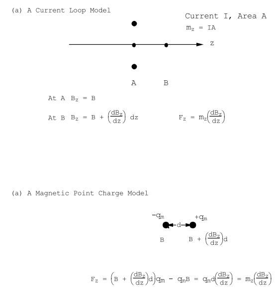
Let us apply the above ideas to calculate the force on a magnetic dipole. Consider a magnetic moment located in an inhomogeneous field that is directed along the z-axis . The magnetic moment can be represented as a small loop carrying a fixed current I, see Figure (5.10). The magnetic moment of the loop, IA, is also directed along z. If the loop moves a distance dz along z, the magnetic field will change from B to B + (dBz/dz)dz. The magnetic energy of the system is given by
UB=L112I2p+L12IpI+L222I2.
During the displacement dz only the mutual inductance coefficient L12 changes: L11 and L22 are not altered. The change in magnetic energy due to the displacement of the loop at constant currents is given by
dUB=IpdL12I=IdΦ.
But
dΦ=AdBz=A(dBzdz)dz,
therefore
dUB=IA(dBzdz)dz.
From an application of Equation (???) one can conclude that the magnetic force on the loop must be
Fx=IA(dBzdz)=mx(dBzdz) Newtons.
This equation for the force on a dipole was derived using arguments based upon circuits in which the currents were held fixed. However, the validity of the expression for the force does not depend upon the manner of its derivation, and Equation (???) is correct for any point dipole.
The result (???) can be generalized by considering displacements along x and y. For a magnetic moment that has only a z-component the result is
→F=mzg→rad(Bz).
The total force acting on a magnetic moment that has components along all three co-ordinate axes is obtained from a further generalization of the above arguments. The result is
→F=mxgr→ad(Bx)+my grad (By)+mzgr→ad(Bz).
The expression (???) can be further transformed by using the fact that curl (→B) = 0 in a homogeneous medium free from currents; because for a current free region curl (→H) = 0, and in a homogeneous permeable region →B=μ→H. From curl (→B) = 0
∂Bx∂y=∂By∂x,∂Bx∂z=∂Bz∂x,∂By∂z=∂Bz∂y.
Using these relations, Equation (???) can be written in the form
Fx=mx∂Bx∂x+my∂Bx∂y+mz∂Bx∂z,
Fy=mx∂By∂x+my∂By∂y+mz∂By∂z,
Fz=mx∂Bz∂x+my∂Bz∂y+mz∂Bz∂z.
or
→F=(→m⋅g→rad)→B.
Equations (???) are the expressions which would be deuced from a magnetic point charge model in which the force on a magnetic pole is given by qm→B (see Figure (5.6.10)), and the dipole is represented by a magnetic charge +qm separated an infinitesimal distance d from a magnetic point charge −qm: the magnetic moment is given by
→m=qmd.
The generalization of Equation (???) to the dipoles contained in a volume element dVol gives the magnetic force per unit volume quoted in Chpt.(1), Section(1.5.1), Equation (1.5.3):
→FM=(→M⋅→∇Bx)ˆux+(→M⋅→∇By)ˆuy+(→M⋅→∇Bz)ˆuz Newtons/m 3.
Here →M is the magnetization per unit volume.
5.6.2 Torque on a Magnetic Dipole.
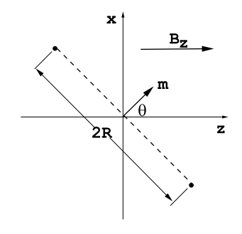
Consider a small current loop placed in a uniform magnetic field generated by a primary coil system carrying a current I1. If the loop is allowed to rotate the flux linkage between it and the primary coil system changes; however, neither its own self-inductance coefficient, L22, nor the self-inductance coefficient of the primary system, L22, changes with the angle of rotation, θ, Figure (5.6.11). The mutual inductance coefficient, L12 = L21, does change with angle, and therefore a small rotation through dθ causes a change in the magnetic energy for fixed currents I1,I2. The change in magnetostatic energy of the system for a small rotation is given by
dUB=I1I2dL12.
The mutual inductance coefficient can be calculated from the flux through the current loop:
Φ2=(πR2)Bzcosθ=(πR2K)I1cosθ.
Therefore
L12=(πR2K)cosθ Henries ,
so that
dL12=−(πR2Ksinθ)dθ.
It follows that the change in the magnetostatic energy of the system as a result of the change in angle is given by
dUB=−(πR2I2)(KI1)sinθdθ.
The change in magnetic energy can be expressed in terms of the magnetic moment of the loop, m, and the value of the magnetic field at the position of the loop (it is assumed that the loop is small enough that the variation of the magnetic field across its diameter can be ignored):
dUB=−Bzmsinθdθ.
This change in the energy must be equal to the external work done by the magnetic torque on the loop (Equation (???)); Tydθ = dUB, where the torque is directed along the y-axis if the rotation takes place in the xz plane, Figure (5.6.11). Therefore
Ty=−mBzsinθ.
The direction of the torque is such as to orient the normal to the plane of the loop along the direction of the applied magnetic field: in other words, the torque is such as to cause both the flux through the loop and the magnetostatic energy to become as large as possible. The magnetic moment associated with the loop is perpendicular to the plane of the loop, consequently Equation (???) can be written in the form
→T=(→m×→B).
The torque (???) can be derived from an effective potential energy
WB=−→m⋅→B Joules ,
using
Tθ=−∂WB∂θ.
Equations (??? and ???) are particularly useful for treating the problem of a collection of permanent dipoles (a permanently magnetized body) that interacts with an applied magnetic field.
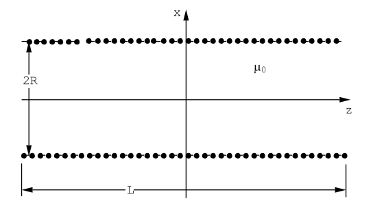
5.6.3 Forces on a Solenoid.
Consider a coil in the form of a very long cylindrical solenoid that is wound with N turns per meter. The length of the solenoid is L meters, and the mean radius of the windings is R meters, Figure (5.6.12). The field at the center of a very long solenoid is given by Equation (4.3.7) of Chpt.(4):
Bz=μ0NI Teslas ,
where the coil carries a current of I Amps. The flux through one turn of the solenoid is ABz = πR2Bz near the center of the solenoid; neglecting end effects which play a relatively small role in the limit L/R → ∞, the total flux through all of the windings is the flux per turn multiplied by the total number of turns
Φ=πR2BzNL,
or
Φ=μ0N2(πR2L)I.
The magnetic energy stored in the field is UB = IΦ/2 Joules, and therefore
UB=μ02N2I2(πR2L).
In order to discuss magnetic forces it is necessary to consider distortions of the solenoid; for example, a change in the length or in its diameter. During those distortions the current will be held fixed. The total number of turns on the solenoid, Ntot = NL, must also remain fixed, and therefore the magnetic energy will be re-written in terms of the total number of turns on the winding:
UB=μ0N2totI2πR22L.
It is apparent from this expression that an increase in solenoid length will reduce the magnetostatic energy, UB. We can conclude that the magnetic forces on the solenoid windings will act in such a way as to shorten the solenoid because any system of coils carrying fixed currents will attempt to arrange themselves so as to maximize the magnetostatic energy of the system. Similarly, any increase in the solenoid radius results in an increase in the magnetostatic energy; it can therefore be concluded that the magnetic forces will place the windings under tension. The magnitude of the magnetic forces can be obtained from an application of Equation (???) which equates the work done by the magnetic forces during a small change in geometry to the increase in magnetic energy. For example, let the length of the solenoid increase by δL; the work done by the magnetic forces is FMδL. The change in magnetic energy for a displacement δL is
δUB=−μ02(N2totL2)I2πR2δL;
consequently, from δUB = FMδL one finds
FM=−(μ0N2I22)πR2 Newtons .
The force that tends to squeeze the turns together is the force that would be generated by a pressure pB = BH/2 Newtons/m2 acting over the crosssectional area of the solenoid.
A similar argument can be used to calculate the tension in the solenoid windings due to magnetic forces. Let the radius of the solenoid of Figure (5.6.12) expand slightly. The work done by a uniform pressure, pM, during this expansion would be
δW=pM(2πR)δR
per meter of length because the work done per unit area of wall per unit length is given by pMδR. The total work done by the magnetic pressure, pM, during the change δR for a cylinder L meters long is given by
δW=pM(2πRL)δR.
The corresponding increase in magnetostatic energy, from Equation (???), is
δUB=μ0N2I2(πRL)δR.
But the work done by the magnetic forces must be equal to the increase in stored magnetic energy if the current is held fixed, and therefore
pM=μ02N2I2=BH2 Newtons /m2.
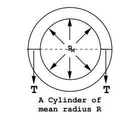
The magnetic field exerts a pressure on the solenoid windings: this pressure results in a tension given by
T=pMR=R(BH2) Newtons/meter ,
see Figure (5.6.13). There are N wires per meter of length, and therefore the tension on each wire will be given by
t=T/N=RN(BH2).
The forces exerted on the windings of a solenoid can be quite large. For example, superconducting solenoids are available that can be used to generate fields in excess of 10 Teslas. The magnetic pressure in a 10 Tesla field is pM = B2/2µ0 = 3.98 × 10⁷ Newtons/m2 . The pressure of one atmosphere is 1.01 × 10⁵ Newtons/m2 , therefore the magnetic pressure associated with a field of 10 Teslas is equivalent to 394 atmospheres. The windings on such a superconducting solenoid must be firmly anchored in order to prevent them from moving