13.7: Chapter 7

Problem (7.1)

In his original experiments on radio waves Hertz used two spheres approximately 0.5 meters in diameter and separated by approximately 0.5 meters. These spheres were charged to a potential difference of 2x10⁵ Volts; as a result one sphere carried a charge of Q₁= +Q= 5.56x10^-6 Coulombs, and the other sphere carried Q₂= -Q Coulombs. The two spheres were suddenly connected together electrically by means of a spark gap (ionized air is an excellent conductor), and the charge oscillated forth and back between the spheres at a frequency which was determined by the geometry but which was of the order of 100 MHz. You may model this system as a point electric dipole oscillating at 100 MHz, where the dipole amplitude is P₀= 2.78x10^-6 Coulomb-meters.

1. Calculate and compare the terms in the expressions for the electric and magnetic fields generated by an oscillating electric dipole as measured at a point in the equatorial plane 1 meter from the dipole (θ= \(\pi\)/2).
2. Calculate and compare the terms in the expressions for the electric and magnetic fields generated by an oscillating electric dipole as measured at a point in the equatorial plane 1 km from the dipole.

Answer (7.1)

\[\text{E}_{\text{T}}=\frac{1}{4 \pi \varepsilon_{0}} 2 \cos \theta\left(\frac{\text{P}_{\text{z}}}{\text{R}^{3}}+\frac{\dot{\text{P}}_{\text{z}}}{\text{CR}^{2}}\right),\nonumber\]

\[\text{E}_{\theta}=\frac{1}{4 \pi \varepsilon_{0}} \sin \theta\left(\frac{\text{P}_{\text{z}}}{\text{R}^{3}}+\frac{\dot{\text{P}}_{\text{z}}}{\text{CR}^{2}}+\frac{\ddot{\text{P}}_{\text{z}}}{\text{c}^{2} \text{R}}\right),\nonumber\]

\[\mathrm{E}_{\phi}=0, \nonumber\]

\[\text{CB}_{\phi}=\frac{1}{4 \pi \varepsilon_{0}} \sin \theta\left(\frac{\dot{\text{P}}_{\text{z}}}{\text{CR}^{2}}+\frac{\ddot{\text{P}}_{\text{z}}}{\text{c}^{2} \text{R}}\right). \nonumber\]

\[\mathrm{B}_{\theta}=\mathrm{B}_{\mathrm{r}}=0, \nonumber\]

At \(\theta=\frac{\pi}{2}\) E_r= 0. For R= 1 meter, f= 10⁸ Hz, ω= 6.28x10⁸ radians/sec

(1) \(\frac{P_{z}}{4 \pi \varepsilon_{0} R^{3}}=2.5 \times 10^{4} \text { Volts/meter. }\)

(2) \(\frac{\dot{P}_{z}}{4 \pi \varepsilon_{0} \quad c R^{2}}=5.2 i \times 10^{4} \quad \text { Volts/meter }\)

(3) \(\frac{\ddot{P}_{z}}{4 \pi \varepsilon_{0} {C}^{2} R}=-1.1 \times 10^{5} \text { Volts/meter }\)

Even at R= 1 meter the field is dominated by the radiation term.

B_\(\phi\) = - (3.7 - 1.7i) x 10^-4 Teslas, i.e. approximately four times the earth's magnetic field.

(b) R= 1 km = 10³ meters.

(1) \(\frac{P_{z}}{4 \pi \varepsilon_{0} R^{3}}=2.5 \times 10^{-5} \text {Volts/meter }\)

(2) \(\frac{\dot{\text{P}}_{\text{z}}}{4 \pi \varepsilon_{0} \text{cR}^{2}}=5.2 \text{ix} 10^{-2} \text {Volts/meter. }\)

(3) \(\frac{\ddot{P}_{z}}{4 \pi \varepsilon_{0} \quad c^{2} R}=-110 \quad \text { Volts/meter }\)

B_\(\phi\) = - 3.67 x 10^-7 Teslas.

Notice that the radiation field is now much larger than the near field components.

Problem (7.2)

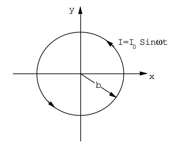
Consider a small current loop of radius b. It carries a current I(t) = I_o sinωt. Calculate the electric and magnetic fields observed at a point P located at R relative to the center of the current loop. There is no net charge density anywhere on the loop i.e. ρ_f ≡ 0. Calculate A for the observer at R(X,Y,Z,t) and keep only the terms to lowest order in (b/R) both in the distance from an element dL on the current loop and in the retarded time \(t_{R}=t-\frac{R}{C}\).

Show that to first order in (b/R) the components of the vector potential are given by

\[\text{A}_{\text{X}}=-\frac{\mu_{0}}{4 \pi} \left(\pi \text{b}^{2} \text{I}_{0}\right)\left(\frac{\text{Y}}{\text{R}}\right)\left(\frac{\operatorname{Sin} \omega(\text{t}-\text{R} / \text{c})}{\text{R}^{2}}+\frac{\omega \operatorname{Cos} \omega(\text{t}-\text{R} / \text{c})}{\text{CR}}\right)\nonumber\]

\[\text{A}_{\text{y}}=\frac{\mu_{0}}{4 \pi} \left(\pi \text{b}^{2} \text{I}_{0}\right)\left(\frac{\text{X}}{\text{R}}\right)\left(\frac{\sin \omega(\text{t}-\text{R} / \text{c})}{\text{R}^{2}}+\frac{\omega \cos \omega(\text{t}-\text{R} / \text{c})}{\text{c} \text{R}}\right)\nonumber\]

or

\[\text{A}_{\phi}=\frac{\mu_{0}}{4 \pi} \left(\pi \text{b}^{2} \text{I}_{0}\right) \sin \theta\left(\frac{\sin \omega(\text{t}-\text{R} / \text{c})}{\text{R}^{2}}+\frac{\omega \cos \omega(\text{t}-\text{R} / \text{c})}{\text{CR}}\right)\nonumber\]

and

A_θ = A_R = 0. Also V = 0 because divA = 0.

Show that for very large R the fields are given by

\[\text{B}_{\theta}=\left(\frac{\mu_{0}}{4 \pi}\right)\left(\pi \text{b}^{2}\right) \frac{\sin \theta}{\text{c}^{2} \text{R}}\left(\frac{\text{d}^{2} \text{I}}{\text{dt}^{2}}\right)_{\text{t}_{\text{R}}}\nonumber\]

\[E_{\phi}=-\left(\frac{\mu_{0}}{4 \pi}\right) \left(\pi b^{2}\right) \frac{\sin \theta}{\operatorname{cR}}\left(\frac{d^{2} I}{d t^{2}}\right)_{t_{R}}\nonumber\]

where \(t_{R}=\left(t-\frac{R}{c}\right)\).

Answer (7.2)

Start from the general expression for the vector potential:

\[\mathbf{A}(\mathbf{R})=\frac{\mu_{0}}{4 \pi} \int \frac{J(\mathbf{r}) d \tau}{|\mathbf{R}-\mathbf{r}|}\nonumber\]

In carrying out the integral the integrand vanishes except on the wire.

\[\therefore \quad \mathbf{A}(\mathbf{R})=\frac{\mu_{0}}{4 \pi} \oint \frac{I\left(t_{R}\right) \mathbf{d l}}{|\mathbf{R}-\mathbf{r}|}\nonumber\]

Now \(\mathbf{d l}=\text { bd } \phi\left[-\sin \phi \hat{\mathbf{u}}_{x}+\cos \phi \hat{\mathbf{u}}_{y}\right]\)

and \(|\mathbf{R}-\mathbf{r}|^{2}=(X-b \cos \phi)^{2}+(Y-b \sin \phi)^{2}+Z^{2}=X^{2}+Y^{2}+Z^{2}-2 b X \cos \phi-2 b \sin \phi Y+b^{2}\)

\(\therefore|\mathbf{R}-\mathbf{r}| \cong R\left[1-\frac{b X \cos \phi}{R^{2}}-\frac{b Y \sin \phi}{R^{2}}\right]\)

Therefore

\[\text{A}_{\text{X}}=\frac{\mu_{0} I_{0}}{4 \pi \text{R}} \int_{0}^{2 \pi}-\operatorname{bsin} \phi d \phi\left[1+\frac{\text{b} \text{X} \cos \phi}{\text{R}^{2}}+\frac{\text{b} \text{Y} \sin \phi}{\text{R}^{2}}\right] \times \sin \omega\left(t-\frac{R}{c}+\frac{b X \cos \phi}{c R}+\frac{b Y \sin \phi}{c R}\right)\nonumber\]

But \(\sin \left[\omega\left(t-\frac{R}{c}\right)+\omega \delta\right]=\cos \omega \delta \sin \omega\left(t-\frac{R}{c}\right)+\sin \omega \delta \cos \omega\left(t-\frac{R}{c}\right)\)

Here \(\delta=\frac{bX \cos \phi}{c R}+\frac{b Y \sin \phi}{c R}\)

and ω\(\delta\) << 1 i.e. of order \(\frac{V}{c}<<1\)

thus \(\cos \omega \delta \cong 1\)

\(\sin \omega \delta \simeq \omega \delta\)

\(\therefore \sin \left[\omega\left(t-\frac{R}{c}\right)+\omega \delta\right]=\sin \omega\left(t-\frac{R}{c}\right)+\omega \delta \cos \omega\left(t-\frac{R}{c}\right)\)

So

\[\text{A}_{\text{X}}=-\frac{\mu_{0}}{4 \pi} \frac{\text{I}_{0} \text{b}}{\text{R}} \int_{0}^{2 \pi} \text{d} \phi \sin \phi\left\{\left(1+\frac{\text{b} \text{X} \cos \phi}{\text{R}^{2}}+\frac{\text{b} \text{Y} \sin \phi}{\text{R}^{2}}\right)\right.\times \left.\left[\sin \omega\left(t-\frac{R}{c}\right)+\cos \omega\left(t-\frac{R}{c}\right) \left(\frac{\omega b \times \cos \phi}{c R}+\frac{\omega b Y \sin \phi}{c R}\right)\right]\right\}\nonumber\]

The only terms which survive the integration over the angles are

\(\text{A}_{\text{x}}=-\frac{\mu_{\text{o}}}{4 \pi}\left(\text{I}_{\text{o}} \pi \text{b}^{2}\right)\left(\frac{\text{Y}}{\text{R}}\right)\left[\frac{\sin \omega\left(\text{t}-\frac{\text{R}}{\text{c}}\right)}{\text{R}^{2}}+\frac{\omega}{\text{c} \text{R}} \cos \omega\left(\text{t}-\frac{\text{R}}{\text{c}}\right)\right]=-\alpha(\text{Y} / \text{R})\)

Similarly

\[\mathrm{A}_{\mathrm{Y}}=\frac{\mu_{0}}{4 \pi} \frac{\mathrm{I}_{0} \mathrm{b}}{\mathrm{R}} \int_{0}^{2 \pi} \mathrm{d} \phi \cos \phi\left[1+\frac{\mathrm{b} \mathrm{X} \cos \phi}{\mathrm{R}^{2}}+\frac{\mathrm{b} \mathrm{Y} \sin \phi}{\mathrm{R}^{2}}\right]\times \sin \omega\left(t-\frac{R}{c}+\frac{b x \cos \phi}{c R}+\frac{b Y \sin \phi}{c R}\right)\nonumber\]

But \(\sin \omega\left(t-\frac{R}{c}+\delta\right)=\cos \omega \delta \sin \omega\left(t-\frac{R}{c}\right)+\sin \omega \delta \cos \omega\left(t-\frac{R}{c}\right)\)

\(\cong\left(\frac{\omega b \times \cos \phi}{c R}+\frac{\omega b Y \sin \phi}{c R}\right) \quad \cos \omega\left(t-\frac{R}{c}\right)+\sin \omega\left(t-\frac{R}{c}\right)\)

\[\begin{array}{l} \therefore A_{Y}=\left(\frac{\mu_{0}}{4 \pi}\right)\left(\frac{I_{0} b}{R}\right) \int_{0}^{2 \pi} d \phi \cos \phi\left\{\left[1+\frac{b X \cos \phi}{R^{2}}+\frac{b Y \sin \phi}{R^{2}}\right] \sin \omega\left(t-\frac{R}{c}\right)\right. \\ \quad \quad \quad \quad+\left(\frac{\omega b X \cos \phi}{c R}+\frac{\omega b Y \sin \phi}{c R}\right) \cos \omega\left(t-\frac{R}{c}\right) \\ \quad \quad \quad \quad+\frac{\mathrm{b} \mathrm{X} \cos \phi}{\mathrm{R}^{2}}\left(\frac{\omega \mathrm{b} \mathrm{X} \cos \phi}{\mathrm{cR}}+\frac{\omega \mathrm{b} \mathrm{Y} \sin \phi}{\mathrm{cR}}\right) \cos \omega\left(t-\frac{\mathrm{R}}{\mathrm{c}}\right) \\ \left.\quad \quad \quad \quad+\frac{\mathrm{b} \mathrm{Y} \sin \phi}{\mathrm{R}^{2}}\left(\frac{\omega \mathrm{b} \mathrm{X} \cos \phi}{\mathrm{cR}}+\frac{\omega \mathrm{b} \mathrm{Y} \sin \phi}{\mathrm{cR}}\right) \cos \omega\left(\mathrm{t}-\frac{\mathrm{R}}{\mathrm{c}}\right)\right\} \end{array} \nonumber\]

The only terms which survive the integration are

\(\text{A}_{\text{y}}=\left(\frac{\mu_{0}}{4 \pi}\right) \left(\text{I}_{\text{O}} \pi \text{b}^{2}\right) \left(\frac{\text{X}}{\text{R}}\right) \left[\frac{\sin \omega(\text{t}-\text{R} / \text{c})}{\text{R}^{2}}+\frac{\omega}{\text{cR}} \cos \omega\left(\text{t}-\frac{\text{R}}{\text{c}}\right)\right]=\alpha(\text{X} / \text{R})\)

But

\[\begin{array}{l}
\frac{X}{R}=\sin \theta \cos \phi \\
\frac{Y}{R}=\sin \theta \sin \phi
\end{array}\nonumber\]

and

\[\begin{array}{l}
\text{A}_{\text{X}}=-\alpha \sin \theta \sin \phi \\
\text{A}_{\text{Y}}=\alpha \sin \theta \cos \phi \\
\text{A}_{\text{z}}=0.
\end{array}\nonumber\]

Since

\[\begin{array}{l}
\hat{\mathbf{u}}_{\text{r}}=(\sin \theta \cos \phi, \sin \theta \sin \phi, \cos \theta) \\
\hat{\mathbf{u}}_{\theta}=(\cos \theta \cos \phi, \cos \theta \sin \phi,-\sin \theta) \\
\hat{\mathbf{u}}_{\phi}=(-\sin \phi, \cos \phi, 0),
\end{array}\nonumber\]

then

\[\mathbf{A} \cdot \hat{\mathbf{u}}_{\text{r}}=0, \quad \mathbf{A} \cdot \hat{\mathbf{u}}_{\theta}=0, \quad \text { and } \quad \mathbf{A} \cdot \hat{\mathbf{u}}_{\phi}=\alpha \sin \theta.\nonumber\]

By comparison with the above one finds

\(\text{A}_{\phi}=\left(\frac{\mu_{0}}{4 \pi}\right)\left(I_{0} \pi \text{b}^{2}\right) \sin \theta\left[\frac{\sin \omega\left(t-\frac{R}{c}\right)}{R^{2}}+\frac{\omega}{c R} \cos \omega\left(t-\frac{R}{c}\right)\right]\)

and A_r = A_θ = 0.

Also V = 0. Let m_o = I_o\(\pi\)b²

\(\operatorname{curl} \mathbf{A}=\frac{1}{r^{2} \sin \theta}\left|\begin{array}{ccc} \hat{\mathbf{u}}_{r} & r \hat{\mathbf{u}}_{\theta} & r \sin \theta \hat{\mathbf{u}}_{\phi} \\ \frac{\partial}{\partial r} & \frac{\partial}{\partial \theta} & \frac{\partial}{\partial \phi} \\ 0 & 0 & r \sin \theta \text{A}_{\phi} \end{array}\right|\)

\(=\left|\begin{array}{cc} \frac{1}{\operatorname{rsin} \theta} \frac{\partial\left(\sin \theta A_{\phi}\right)}{\partial \theta} \\ -\frac{1}{r} \frac{\partial\left(r A_{\phi}\right)}{\partial r} \\ 0 \end{array}\right|\)

\(\begin{aligned} \therefore B_{r} &=\frac{1}{r \sin \theta} \frac{\partial}{\partial \theta}\left(\sin \theta \quad A_{\phi}\right) \\ &=\left(\frac{\mu_{0}}{4 \pi}\right) \frac{2 m_{0} \cos \theta}{R}\left[\frac{\sin \omega\left(t-\frac{R}{c}\right)}{R^{2}}+\frac{\omega}{c R} \cos \omega\left(t-\frac{R}{c}\right)\right] \end{aligned}\)

\(\text{B}_{\theta}=\left(\frac{\mu_{0}}{4 \pi}\right) \text{m}_{0} \sin \theta\left[\frac{\sin \omega\left(t-\frac{\text{R}}{\text{c}}\right)}{\text{R}^{3}}+\frac{\omega}{\text{cR}^{2}} \cos \omega\left(t-\frac{\text{R}}{\text{c}}\right)\right.\left.-\frac{\omega^{2}}{c^{2} R} \sin \omega\left(t-\frac{R}{c}\right)\right]\)

\(\text{B}_{\phi}=0\)

\(E_{\phi}=-\frac{\partial A_{\phi}}{\partial t}=-\left(\frac{\mu_{0}}{4 \pi}\right) m_{0} \sin \theta \quad\left[\frac{\omega}{R^{2}} \cos \omega\left(t-\frac{R}{c}\right)-\frac{\omega^{2}}{c R} \sin \omega\left(t-\frac{R}{c}\right)\right]\)

and E_r = E_θ = 0.

For large R only the terms in 1/R are important.

\(\text{B}_{\theta}=\left(\frac{\mu_{0}}{4 \pi}\right) \pi \text{b}^{2} \sin \theta \left(-\frac{\omega^{2}}{\text{c}^{2} \text{R}}\right) \text{I}_{0} \sin \omega\left(\text{t}-\frac{\text{R}}{\text{c}}\right)\)

\(B_{\theta}=\left(\frac{\mu_{0}}{4 \pi}\right) \frac{\pi b^{2} \sin \theta}{c^{2} R}\left(\frac{d^{2} I}{d t^{2}}\right)_{t_{R}}\)

Similarly

\(E_{\phi}=-\left(\frac{\mu_{0}}{4 \pi}\right) \frac{\pi b^{2} \sin \theta}{\operatorname{cR}}\left(\frac{d^{2} I}{d t^{2}}\right)_{t_{R}} \quad \quad \quad \text { ie } \cdot E_{\phi}=-c B_{\theta}\)

Problem (7.3).

A magnetic dipole transmitter consists of 10 turns of wire wound on a form whose radius is 10 cm. An alternating current whose amplitude is 100 Amps and whose frequency is 100 MHz is passed through the coil.

(a) What is the maximum magnetic moment of the above coil?

(b) Assuming that the above coil can be approximated by a point magnetic dipole, calculate and compare the terms in the expressions for the electric and magnetic fields generated by an oscillating magnetic dipole as measured at a point in the equatorial plane 1 meter from the dipole (θ= \(\pi\)/2).

(c) Calculate and compare the terms in the expressions for the electric and magnetic fields generated by an oscillating magnetic dipole as measured at a point in the equatorial plane 1 km from the dipole.

Answer (7.3)

(a) The maximum magnetic moment is m_z= IA , or in this case m_z= (1000)(.01\(\pi\))= 31.4 Amp.m².

(b) The fields generated by an oscillating magnetic dipole are given by

\[\text{B}_{\text{r}}=\frac{\mu_{0}}{4 \pi} 2 \cos \theta\left(\frac{\text{m}_{\text{z}}}{\text{R}^{3}}+\frac{\dot{\text{m}}_{\text{z}}}{\text{cR}^{2}}\right)\nonumber\]

\[\text{B}_{\theta}=\frac{\mu_{0}}{4 \pi} \sin \theta\left(\frac{\text{m}_{\text{z}}}{\text{R}^{3}}+\frac{\dot{\text{m}}_{\text{z}}}{\text{cR}^{2}}+\frac{\ddot{\text{m}_{\text{z}}}}{\text{c}^{2} \text{R}}\right)\nonumber\]

\[\text{B}_{\phi}=0\nonumber\]

\[\text{E}_{\phi}=-\text{c}\left(\frac{\mu_{0}}{4 \pi} \sin \theta\left(\frac{\dot{\text{m}}_{\text{z}}}{\text{cR}^{2}}+\frac{\ddot{\text{m}_{\text{z}}}}{\text{c}^{2} \text{R}}\right)\right)\nonumber\]

\[\text{E}_{\text{r}}=\text{E}_{\theta}=0\nonumber\]

For this problem θ= \(\pi\)/2, Cosθ=0 and Sinθ=1. Also R= 1 meter and ω= 2\(\pi\)f = 6.28x10⁸ radians/sec.

(1) \(\frac{\mu_{0}}{4 \pi} \frac{m_{z}}{R^{3}}=3.14 \times 10^{-6} \text {Teslas }\)

(2) \(\frac{\mu_{0}}{4 \pi} \frac{\dot{\text{m}}_{\text{z}}}{\text{cR}^{2}}=6.58 \text{ix} 10^{-6} \text{Tes} 1 \text{as}\)

since \(\frac{\dot{m}_{z}}{c}=\frac{i \omega m_{z}}{c}=65.80 i\)

(3) \(\frac{\mu_{0}}{4 \pi} \frac{\ddot{m}_{z}}{c^{2} R}=-13.78 \times 10^{-6} \text {Teslas }\)

since \(\ddot{m}_{z}=-\omega^{2} m_{z}=-1.24 \times 10^{19}\), and \(E_{\phi}=(4134-1970 i) \text{Volts/meter.}\)

(c) For R= 1 km = 10³ meters

(1) \(\frac{\mu_{0}}{4 \pi} \frac{\text{m}_{\text{z}}}{\text{R}^{3}}=3.14 \times 10^{-15} \text {Teslas }\).

(2) \(\frac{\mu_{0}}{4 \pi} \frac{\dot{\text{m}}_{\text{z}}}{\text{cR}^{2}}=6.58 \text{ix} 10^{-12} \text{Tes} 1 \text{as}\).

(3) \(\frac{\mu_{0}}{4 \pi} \frac{\ddot{m}_{z}}{c^{2} R}=-13.78 \times 10^{-9} \text {Teslas }\), and \(E_{\phi}=\left(4.13-1.97 \text{ix} 10^{-3}\right) \text {Volts/meter. }\)

Problem (7.4).

An electron is at rest at the origin of co-ordinates. It is suddenly given an acceleration of a = 1.76 x 10¹⁷ m/sec² for 10^-14 seconds after which it continues with a uniform velocity. This acceleration, which is directed along the z axis, was produced by a 1000 V pulse applied across a gap of 1 mm at t = 0. An observer is located at X = 1 meter, Y= Z= 0 m.

(a) Make a sketch showing how the x-component of the electric field measured by the observer varies with time (observer's time--his clock is synchronized with that at the origin).

(b) Ditto showing how E_z varies with time.

Answer (7.4).

Think of putting both a stationary charge of +1.6x10^-19 C. and a stationary charge of - 1.6x10^-19 C. at the origin: the net charge is zero so that these together add nothing to the fields. However, the + charge and the moving electron together form a dipole p_z= - qz(t) where q= 1.6x10^-19 C. The time varying dipole generates the fields

\[E_{r}=\frac{1}{4 \pi \varepsilon_{0}} 2 \cos \theta\left(\frac{p_{z}}{R^{3}}+\frac{\dot{p}_{z}}{c R^{2}}\right)\nonumber\]

\[\text{E}_{\theta}=\frac{1}{4 \pi \varepsilon_{0}} \sin \theta \quad\left(\frac{\text{p}_{2}}{\text{R}^{3}}+\frac{\dot{\text{p}}_{2}}{\text{cR}^{2}}+\frac{\ddot{\text{p}}_{2}}{\text{c}^{2} \text{R}}\right).\nonumber\]

The left over static charge at the origin generates the static field

\[E_{X}=\frac{1}{4 \pi \varepsilon_{0}} \frac{-q}{R^{2}}\nonumber\]

at R= (1,0,0).

The time scale T₀ for this problem is the time required for light to travel 1 m; T₀= 3.33x10^-9 seconds. The velocity of the electron after the acceleration is V= 1.76x10³ m/sec. Therefore on the time scale of interest here the electron has moved only VT₀= 5.9x10^-6 meters, thus the change in position is negligible compared with the observer distance of 1 m. over the time scales of interest here (~10^-8 secs., z= 1.76x10^-5 m), one finds

\[\mathrm{p}_{\mathrm{z}}=-\left(1.6 \times 10^{-19}\right)\left(1.76 \times 10^{-5}\right)=-2.82 \times 10^{-24} \mathrm{Cm}.\nonumber\]

\[\frac{\dot{p}_{z}}{c}=-0.94 \times 10^{-24} \text{C}.\nonumber\]

\[\frac{\dot{p}_{z}}{c^{2}}=-3.13 \times 10^{-19} \mathrm{C} / \mathrm{m}, \text { during the acceleration. }\nonumber\]

These fields are directed along +z for an observer at R= (1,0,0). It is clear therefore that the acceleration spike in E_z will be very large compared with the other two terms in E_θ.

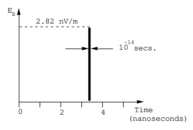
The observer at (1,0,0) will see a steady field of E_x= - 14.4x10^-10 V/m. An electric field spike will be observed beginning at T₀= 3.33x10^-9 secs after the impulse: this spike E_z= 28.2x10^-10 V/m will last for 10^-14 secs. After the spike has passed the component E_z will remain at the level of 8.46x10^-15 V/m. over the time scale of interest here. It is clear that this residual component is very small compared with the radiation spike.

In summary: the acceleration field of 282 x 10^-9 V/m which lasts 10^-14 seconds is directed along \(-\hat{\mathbf{u}}_{\theta}\) because the charge is negative. Therefore for an observer at P(1,0,0) the electric field is directed along z. The acceleration begins at t=0. However, the time required for the field to reach the observer is \(\frac{1}{c}=3.33 \times 10^{-9}\) seconds (a distance of 1 meter at the velocity of light). Therefore at t = 3.33 x 10^-9 seconds the observer will see a transverse pulse which lasts 10^-14 secs. This is superposed on a steady electric field of E_x = -14.4x10^-10 V/m. (Steady on the time-scale of interest here.)

Problem (7.5).

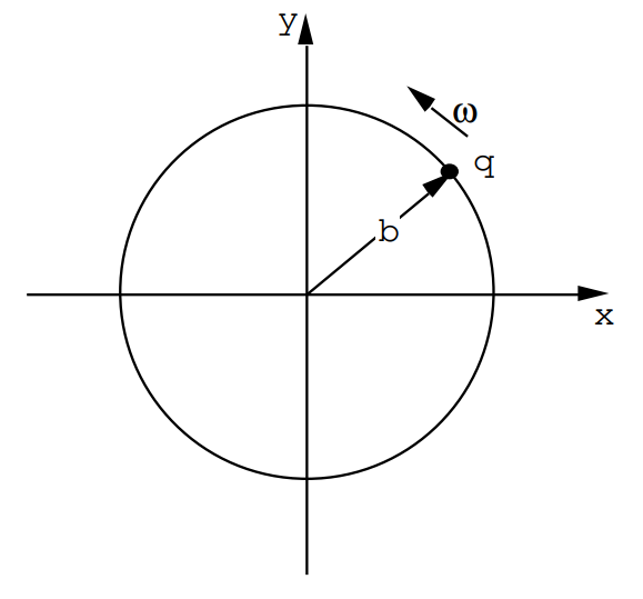
A particle carrying a charge q revolves in a circle at a constant speed v = bω. This motion can be decomposed into two coupled motions

\[\begin{array}{l} x=b \cos \omega t \\ y=b \sin \omega t \end{array}\nonumber\]

Let b be very small compared with the distance to the observer so that this radiation source can be treated like two orthogonal point dipoles qx and qy.

(a) Consider an observer at P = (R,0,0). Show that this observer will see a radiation field polarized along y and given by

\(E_{y}=\frac{\text{qb} \omega^{2} \sin \omega(\text{t}-\text{R} / \text{c})}{4 \pi \varepsilon_{\text{o}} \text{c}^{2} \text{R}} \quad \text{Volts} / \text{m}.\)

(b) Consider an observer at P = (0,R,0). Show that this observer will see a radiation field polarized along x and given by

\(E_{x}=\frac{\text{qb} \omega^{2} \cos \omega(\text{t}-\text{R} / \text{C})}{4 \pi \varepsilon_{\text{o}} \text{c}^{2} \text{R}} \quad \text{Volts} / \text{m}.\)

(c) Consider an observer at P = (0,0,R). Show that this observer will see circularly polarized light whose electric field components are given by

\(\text{E}_{\text{X}}=\frac{\text{qb} \omega^{2} \cos \omega(\text{t}-\text{R} / \text{c})}{4 \pi \varepsilon_{\text{O}} \text{c}^{2} \text{R}} \quad \text { Volts / m. }\)

\(\text{E}_{\text{y}}=\frac{\text{qb} \omega^{2} \sin \omega(\text{t}-\text{R} / \text{c})}{4 \pi \varepsilon_{\text{o}} \text{c}^{2} \text{R}} \quad \text { Volts /m. }\)

Answer (7.5).

This motion can be regarded as a superposition of two linear motions. The electric field (radiation field) amplitude produced by an accelerated charge is given by

\(\text{E}_{\theta}=\frac{1}{4 \pi \varepsilon_{\text{o}}} \frac{\text{qa} \sin \theta}{\text{c}^{2} \text{r}}=\frac{1}{4 \pi \varepsilon_{0}} \frac{\ddot{\text{p}} \sin \theta}{\text{c}^{2} \text{r}}\), a evaluated at t_R = t - R/c For each of the above cases θ = \(\pi\)/2

\(\therefore \text{E}_{\theta}=\frac{\text{qa}}{4 \pi \varepsilon_{\circ} \text{c}^{2} \text{r}}\)

The above results follow immediately since a_x = -bω² cosωt and a_y = - bω² sinωt. The observer at (R,0,0) will see radiation only due to p_y. The observer at (0,R,0) will see radiation only due to p_x. The observer at (0,0,R) will see radiation from both p_x and p_y. The observer located along the z-axis will see circularly polarized radiation because if

\[\text{E}_{\text{X}}=\text{E}_{0} \cos \omega\left(\text{t}-\frac{\text{R}}{\text{c}}\right),\nonumber\]

and

\[\text{E}_{\text{y}}=\text{E}_{0} \sin \omega\left(\text{t}-\frac{\text{R}}{\text{c}}\right),\nonumber\]

these two fields together form a vector of fixed magnitude E₀ rotating at the angular frequency ω.