2.4: A Point Charge and an Infinite Conducting Plane

An infinite plane metal plate is in the $xy$-plane. A point charge +$Q$ is placed on the $z$-axis at a height $h$ above the plate. Consequently, electrons will be attracted to the part of the plate immediately below the charge, so that the plate will carry a negative charge density $σ$ which is greatest at the origin and which falls off with distance $\rho$ from the origin. Can we determine $σ(\rho)$? See Figure $II.2$

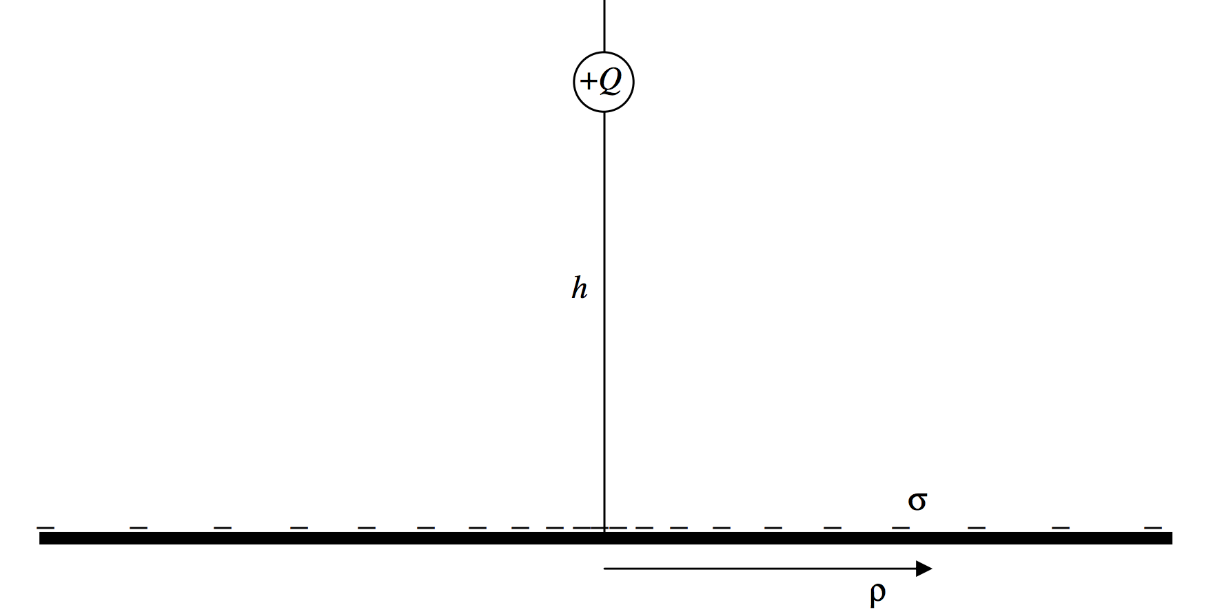
$\text{FIGURE II.2}$

First, note that the metal surface, being a conductor, is an equipotential surface, as is any metal surface. The potential is uniform anywhere on the surface. Now suppose that, instead of the metal surface, we had (in addition to the charge +$Q$ at a height $h$ above the $xy$-plane), a second point charge, −$Q$, at a distance $h$ below the $xy$-plane. The potential in the $xy$-plane would, by symmetry, be uniform everywhere. That is to say that the potential in the $xy$-plane is the same as it was in the case of the single point charge and the metal plate, and indeed the potential at any point above the plane is the same in both cases. For the purpose of calculating the potential, we can replace the metal plate by an image of the point charge. It is easy to calculate the potential at a point $(z , \rho)$. If we suppose that the permittivity above the plate is $\epsilon_0$, the potential at $(z , \rho)$ is

$$\label{2.4.1}V=\frac{Q}{4\pi\epsilon_0}\left ( \frac{1}{[\rho^2+(h-z)^2]^{1/2}}-\frac{1}{[\rho^2+(h+z)^2]^{1/2}}\right )$$

The field strength $E$ in the $xy$-plane is -$∂V/ ∂z$ evaluated at $z = 0$, and this is

$$\label{2.4.2}E=-\frac{2Q}{4\pi\epsilon_0}\cdot \frac{h}{(\rho^2+h^2)^{3/2}}.$$

The $D$-field is $\epsilon_0$ times this, and since all the lines of force are above the metal plate, Gauss's theorem provides that the charge density is $σ = D$, and hence the charge density is

$$\label{2.4.3}\sigma=-\frac{Q}{2\pi}\cdot \frac{h}{(\rho^2+h^2)^{3/2}}.$$

This can also be written

$$\label{2.4.4}\sigma = -\frac{Q}{2\pi}\cdot \frac{h}{ξ^3},$$

where $ξ^2=\rho^2+h^2$, with obvious geometric interpretation.

Exercise: How much charge is there on the surface of the plate within an annulus bounded by radii $\rho$ and $\rho + d\rho$? Integrate this from zero to infinity to show that the total charge induced on the plate is −$Q$.