
2.6: Two Semicylindrical Electrodes
- Page ID
- 5422

\( \newcommand{\vecs}[1]{\overset { \scriptstyle \rightharpoonup} {\mathbf{#1}} } \)
\( \newcommand{\vecd}[1]{\overset{-\!-\!\rightharpoonup}{\vphantom{a}\smash {#1}}} \)
\( \newcommand{\id}{\mathrm{id}}\) \( \newcommand{\Span}{\mathrm{span}}\)
( \newcommand{\kernel}{\mathrm{null}\,}\) \( \newcommand{\range}{\mathrm{range}\,}\)
\( \newcommand{\RealPart}{\mathrm{Re}}\) \( \newcommand{\ImaginaryPart}{\mathrm{Im}}\)
\( \newcommand{\Argument}{\mathrm{Arg}}\) \( \newcommand{\norm}[1]{\| #1 \|}\)
\( \newcommand{\inner}[2]{\langle #1, #2 \rangle}\)
\( \newcommand{\Span}{\mathrm{span}}\)
\( \newcommand{\id}{\mathrm{id}}\)
\( \newcommand{\Span}{\mathrm{span}}\)
\( \newcommand{\kernel}{\mathrm{null}\,}\)
\( \newcommand{\range}{\mathrm{range}\,}\)
\( \newcommand{\RealPart}{\mathrm{Re}}\)
\( \newcommand{\ImaginaryPart}{\mathrm{Im}}\)
\( \newcommand{\Argument}{\mathrm{Arg}}\)
\( \newcommand{\norm}[1]{\| #1 \|}\)
\( \newcommand{\inner}[2]{\langle #1, #2 \rangle}\)
\( \newcommand{\Span}{\mathrm{span}}\) \( \newcommand{\AA}{\unicode[.8,0]{x212B}}\)
\( \newcommand{\vectorA}[1]{\vec{#1}} % arrow\)
\( \newcommand{\vectorAt}[1]{\vec{\text{#1}}} % arrow\)
\( \newcommand{\vectorB}[1]{\overset { \scriptstyle \rightharpoonup} {\mathbf{#1}} } \)
\( \newcommand{\vectorC}[1]{\textbf{#1}} \)
\( \newcommand{\vectorD}[1]{\overrightarrow{#1}} \)
\( \newcommand{\vectorDt}[1]{\overrightarrow{\text{#1}}} \)
\( \newcommand{\vectE}[1]{\overset{-\!-\!\rightharpoonup}{\vphantom{a}\smash{\mathbf {#1}}}} \)
\( \newcommand{\vecs}[1]{\overset { \scriptstyle \rightharpoonup} {\mathbf{#1}} } \)
\( \newcommand{\vecd}[1]{\overset{-\!-\!\rightharpoonup}{\vphantom{a}\smash {#1}}} \)
\(\newcommand{\avec}{\mathbf a}\) \(\newcommand{\bvec}{\mathbf b}\) \(\newcommand{\cvec}{\mathbf c}\) \(\newcommand{\dvec}{\mathbf d}\) \(\newcommand{\dtil}{\widetilde{\mathbf d}}\) \(\newcommand{\evec}{\mathbf e}\) \(\newcommand{\fvec}{\mathbf f}\) \(\newcommand{\nvec}{\mathbf n}\) \(\newcommand{\pvec}{\mathbf p}\) \(\newcommand{\qvec}{\mathbf q}\) \(\newcommand{\svec}{\mathbf s}\) \(\newcommand{\tvec}{\mathbf t}\) \(\newcommand{\uvec}{\mathbf u}\) \(\newcommand{\vvec}{\mathbf v}\) \(\newcommand{\wvec}{\mathbf w}\) \(\newcommand{\xvec}{\mathbf x}\) \(\newcommand{\yvec}{\mathbf y}\) \(\newcommand{\zvec}{\mathbf z}\) \(\newcommand{\rvec}{\mathbf r}\) \(\newcommand{\mvec}{\mathbf m}\) \(\newcommand{\zerovec}{\mathbf 0}\) \(\newcommand{\onevec}{\mathbf 1}\) \(\newcommand{\real}{\mathbb R}\) \(\newcommand{\twovec}[2]{\left[\begin{array}{r}#1 \\ #2 \end{array}\right]}\) \(\newcommand{\ctwovec}[2]{\left[\begin{array}{c}#1 \\ #2 \end{array}\right]}\) \(\newcommand{\threevec}[3]{\left[\begin{array}{r}#1 \\ #2 \\ #3 \end{array}\right]}\) \(\newcommand{\cthreevec}[3]{\left[\begin{array}{c}#1 \\ #2 \\ #3 \end{array}\right]}\) \(\newcommand{\fourvec}[4]{\left[\begin{array}{r}#1 \\ #2 \\ #3 \\ #4 \end{array}\right]}\) \(\newcommand{\cfourvec}[4]{\left[\begin{array}{c}#1 \\ #2 \\ #3 \\ #4 \end{array}\right]}\) \(\newcommand{\fivevec}[5]{\left[\begin{array}{r}#1 \\ #2 \\ #3 \\ #4 \\ #5 \\ \end{array}\right]}\) \(\newcommand{\cfivevec}[5]{\left[\begin{array}{c}#1 \\ #2 \\ #3 \\ #4 \\ #5 \\ \end{array}\right]}\) \(\newcommand{\mattwo}[4]{\left[\begin{array}{rr}#1 \amp #2 \\ #3 \amp #4 \\ \end{array}\right]}\) \(\newcommand{\laspan}[1]{\text{Span}\{#1\}}\) \(\newcommand{\bcal}{\cal B}\) \(\newcommand{\ccal}{\cal C}\) \(\newcommand{\scal}{\cal S}\) \(\newcommand{\wcal}{\cal W}\) \(\newcommand{\ecal}{\cal E}\) \(\newcommand{\coords}[2]{\left\{#1\right\}_{#2}}\) \(\newcommand{\gray}[1]{\color{gray}{#1}}\) \(\newcommand{\lgray}[1]{\color{lightgray}{#1}}\) \(\newcommand{\rank}{\operatorname{rank}}\) \(\newcommand{\row}{\text{Row}}\) \(\newcommand{\col}{\text{Col}}\) \(\renewcommand{\row}{\text{Row}}\) \(\newcommand{\nul}{\text{Nul}}\) \(\newcommand{\var}{\text{Var}}\) \(\newcommand{\corr}{\text{corr}}\) \(\newcommand{\len}[1]{\left|#1\right|}\) \(\newcommand{\bbar}{\overline{\bvec}}\) \(\newcommand{\bhat}{\widehat{\bvec}}\) \(\newcommand{\bperp}{\bvec^\perp}\) \(\newcommand{\xhat}{\widehat{\xvec}}\) \(\newcommand{\vhat}{\widehat{\vvec}}\) \(\newcommand{\uhat}{\widehat{\uvec}}\) \(\newcommand{\what}{\widehat{\wvec}}\) \(\newcommand{\Sighat}{\widehat{\Sigma}}\) \(\newcommand{\lt}{<}\) \(\newcommand{\gt}{>}\) \(\newcommand{\amp}{&}\) \(\definecolor{fillinmathshade}{gray}{0.9}\)This section requires that the reader should be familiar with functions of a complex variable and conformal transformations. For readers not familiar with these, this section can be skipped without prejudice to understanding following chapters. For readers who are familiar, this is a nice example of conformal transformations to solve a physical problem.
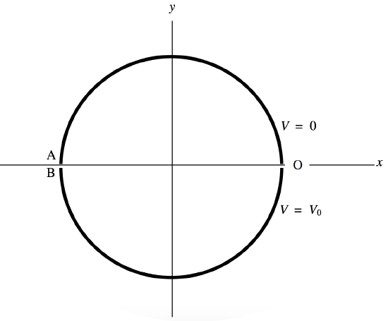
\(\text{FIGURE II.5}\)
We have two semicylindrical electrodes as shown in Figure \(II\).5. The potential of the upper one is 0 and the potential of the lower one is \(V_0\). We'll suppose the radius of the circle is 1; or, what amounts to the same thing, we'll express coordinates \(x\) and \(y\) in units of the radius. Let us represent the position of any point whose coordinates are (x , y) by a complex number \(z = x + iy\).
Now let \(w = u + iv\) be a complex number related to \(z\) by \(w=i\left (\frac{1-z}{1+z}\right )\); that is, \(z=\frac{1+ iw}{1- iw}\). Substitute \(w = u + iv \text{ and }z = x + iy\) in each of these equations, and equate real and imaginary parts, to obtain
\[\begin{align}\label{2.6.1}u&=\frac{2y}{(1+x)^2+y^2};\quad\quad &&v=\frac{1-x^2+y^2}{(1+x)^2+y^2};\\ x&=\frac{1-u^2-v^2}{u^2+(1+v)^2}; &&y=\frac{2u}{u^2+(1+v)^2}.\label{2.6.2}\end{align}\]
In that case, the upper semicircle \((V = 0)\) in the \(xy\)-plane maps on to the positive \(u\)-axis in the \(uv\)-plane, and the lower semicircle \((V = V_0)\) in the \(xy\)-plane maps on to the negative \(u\)-axis in the \(uv\)-plane. (Figure \(II\).6.) Points inside the circle bounded by the electrodes in the \(xy\)-plane map on to points above the \(u\)-axis in the \(uv\)-plane.
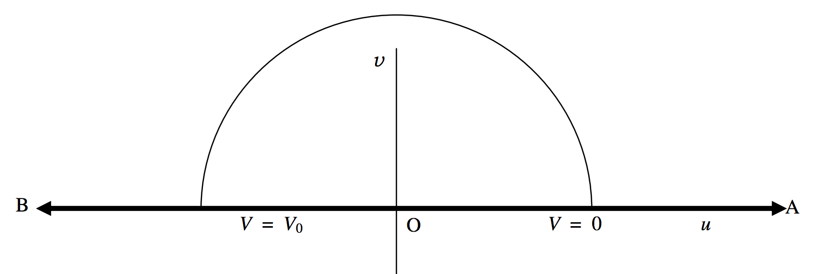
\(\text{FIGURE II.6}\)
In the \(uv\)-plane, the lines of force are semicircles, such as the one shown. The potential goes from 0 at one end of the semicircle to \(V_0\) at the other, and so equation to the semicircular line of force is
\[\label{2.6.3}\frac{V}{V_0}=\frac{\text{arg}\,w}{\pi}\]
or
\[\label{2.6.4}V=\frac{V_0}{\pi}\tan^{-1}(v/u).\]
The equipotentials (\(V\) = constant) are straight lines in the \(uv\)-plane of the form
\[\label{2.6.5}v=fu.\]
(You would prefer me to use the symbol \(m\) for the slope of the equipotentials, but in a moment you will be glad that I chose the symbol \(f\).)
If we now transform back to the \(xy\)-plane, we see that the equation to the lines of force is
\[\label{2.6.6}V=\frac{V_0}{\pi}\tan^{-1} \left (\frac{1-x^2-y^2}{2y}\right ).\]
and the equation to the equipotentials is
\[\label{2.6.7}1-x^2-y^2=2fy,\]
or
\[\label{2.6.8}x^2+y^2+2fy-1=0\]
Now aren't you glad that I chose \(f\) ? Those who are handy with conic sections (see Chapter 2 of Celestial Mechanics) will understand that the equipotentials in the \(xy\)-plane are circles of radii \(\sqrt{f^2 + 1}\), whose centres are at \((0 , \pm f )\), and which all pass through the points \((\pm 1 , 0)\). They are drawn as blue lines in Figure \(II\).7. The lines of force are the orthogonal trajectories to these, and are of the form
\[\label{2.6.9}x^2+y^2+2gy+1=0\]
These are circles of radii \(\sqrt{g^2 −1}\) and have their centres at \((0 , \pm g)\). They are shown as dashed red lines in Figure \(II\).7.
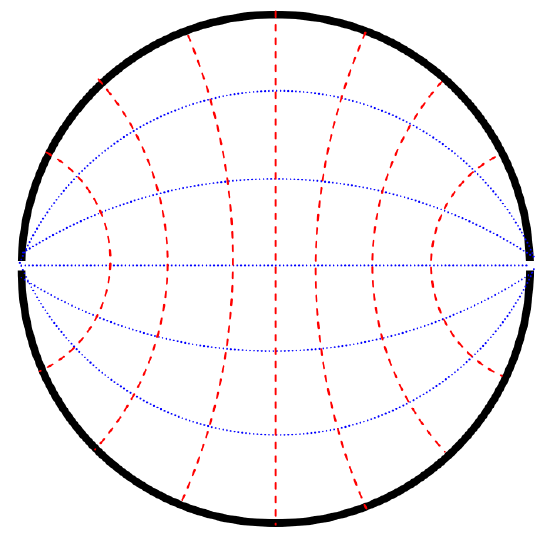
\(\text{FIGURE II.7}\)