
6.11: Ampère’s Theorem


- Last updated
- Mar 5, 2022
- Save as PDF

( \newcommand{\kernel}{\mathrm{null}\,}\)
In Section 1.9 we introduced Gauss’s theorem, which is that the total normal component of the D-flux through a closed surface is equal to the charge enclosed within that surface. Gauss’s theorem is a consequence of Coulomb’s law, in which the electric field from a point source falls off inversely as the square of the distance. We found that Gauss’s theorem was surprisingly useful in that it enabled us almost immediately to write down expressions for the electric field in the vicinity of various shapes of charged bodies without going through a whole lot of calculus.
Is there perhaps a similar theorem concerned with the magnetic field around a current-carrying conductor that will enable us to calculate the magnetic field in its vicinity without going through a lot of calculus? There is indeed, and it is called Ampère’s Theorem.
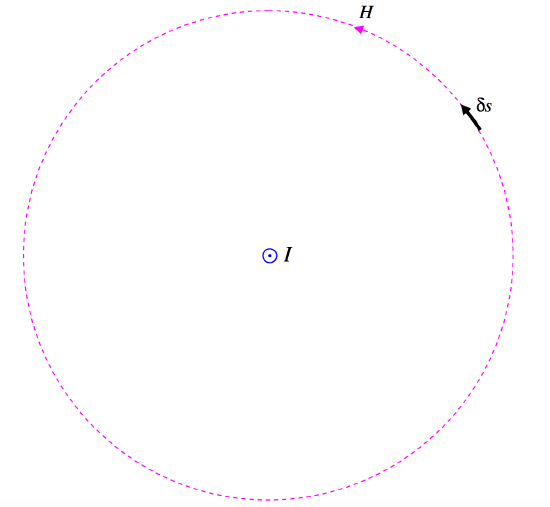
FIGURE VI.9
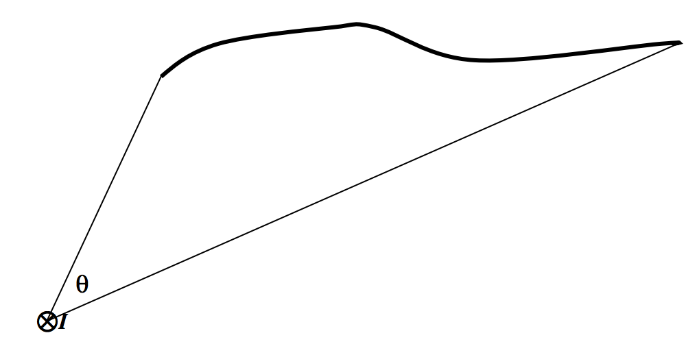
In Figure VI.9 there is supposed to be a current Icoming towards you in the middle of the circle. I have drawn one of the magnetic field lines – a dashed line of radius r. The strength of the field there is H=I/(2πr). I have also drawn a small elemental length ds on the circumference of the circle. The line integral of the field around the circle is just H times the circumference of the circle. That is, the line integral of the field around the circle is just I. Note that this is independent of the radius of the circle. At greater distances from the current, the field falls off as 1/r, but the circumference of the circle increases as r, so the product of the two (the line integral) is independent of r.
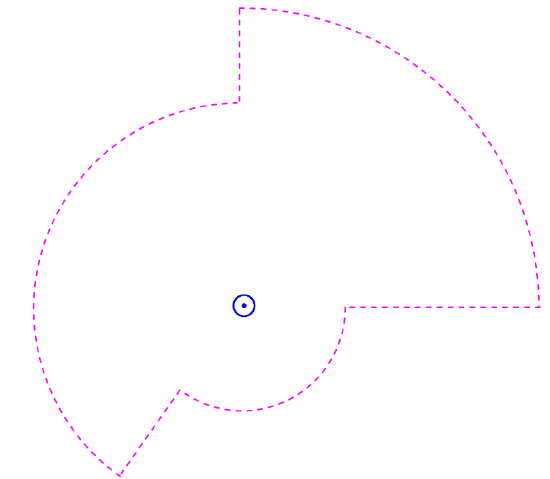
FIGURE VI.10
Consequently, if I calculate the line integral around a circuit such as the one shown in Figure VI.10, it will still come to just I. Indeed it doesn’t matter what the shape of the path is. The line integral is ∫H⋅ds. The field H at some point is perpendicular to the line joining the current to the point, and the vector ds is directed along the path of integration, and H⋅ds is equal to H times the component of ds along the direction of H, so that, regardless of the length and shape of the path of integration:
The line integral of the field H around any closed path is equal to the current enclosed by that path.
This is Ampère’s Theorem.
So now let’s do the infinite solenoid again. Let us calculate the line integral around the rectangular amperian path shown in Figure VI.11. There is no contribution to the line integral along the vertical sides of the rectangle because these sides are perpendicular to the field, and there is no contribution from the top side of the rectangle, since the field there is zero (if the solenoid is infinite). The only contribution to the line integral is along the bottom side of the rectangle, and the line integral there is just Hl, where l is the length of the rectangle. If the number of turns of wire per unit length along the solenoid is n, there will be nl turns enclosed by the rectangle, and hence the current enclosed by the rectangle is nlI, where I is the current in the wire. Therefore by Ampère’s theorem, Hl=nlI, and so H=nI, which is what we deduced before rather more laboriously. Here H is the strength of the field at the position of the lower side of the rectangle; but we can place the rectangle at any height, so we see that the field is nI anywhere inside the solenoid. That is, the field inside an infinite solenoid is uniform.
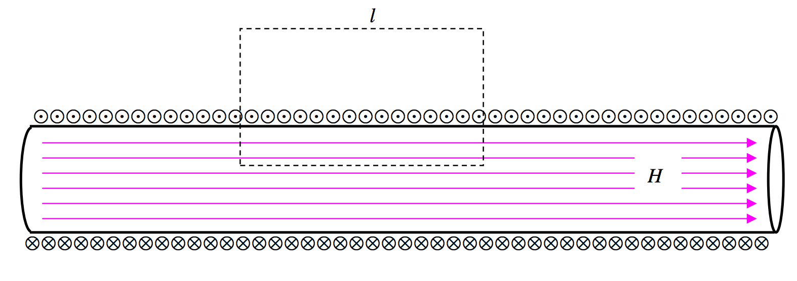
FIGURE VI.11
It is perhaps worth noting that Gauss’s theorem is a consequence of the inverse square diminution of the electric field with distance from a point charge, and Ampère’s theorem is a consequence of the inverse first power diminution of the magnetic field with distance from a line current.
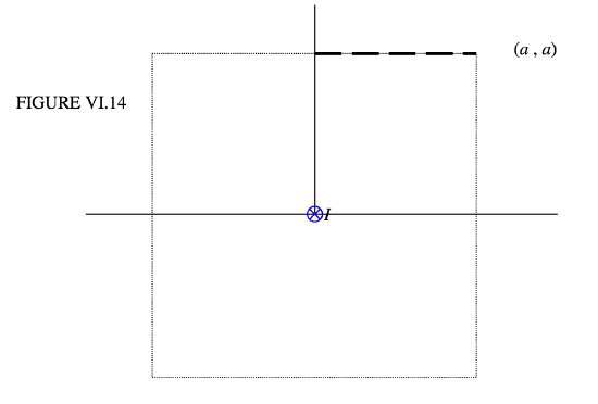
from the axis, r<a?
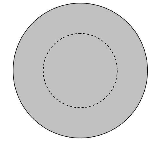
FIGURE VI.15
Figure VI.15 shows the cross-section of the rod, and I have drawn an amperian circle of radius r. If the field at the circumference of the circle is H, the line integral around the circle is 2πrH. The current enclosed within the circle is Ir2/a2. These two are equal, and therefore H=Ir/(2πa2).
More and More Examples
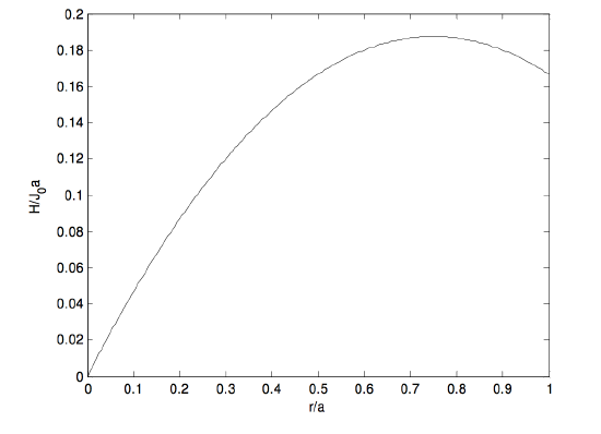
In the above example, the current density was uniform. But now we can think of lots and lots of examples in which the current density is not uniform. For example, let us imagine that we have a long straight hollow cylindrical tube of radius a, perhaps a linear particle accelerator, and the current density J (amps per square metre) varies from the middle (axis) of the cylinder to its edge according to J(r)=J0(1−r/a). The total current is, of course, I=2π∫a0J(r)rdr=13πa2J0 and the mean current density is ¯J=13J0.
The question, however, is: what is the magnetic field H at a distance r from the axis? Further, show that the magnetic field at the edge (circumference) of the cylinder is 16J0a, and that the field reaches a maximum value of 316J0a at r=34a.
Well, the current enclosed within a distance r from the axis is
I=2π∫r0J(x)xdx=πJ0r2(1−2r3a),
and this is equal to the line integral of the magnetic field around a circle of radius r, which is 2πrH. Thus
H=12J0r(1−2r3a).
At the circumference of the cylinder, this comes to 16J0a. Calculus shows that H reaches a maximum value of 316J0a at r=34a. The graph below shows H/(J0a) as a function of x/a.
Having whetted our appetites, we can now try the same problem but with some other distributions of current density, such as
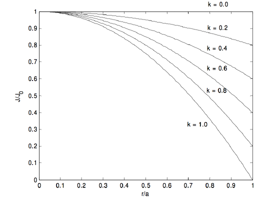
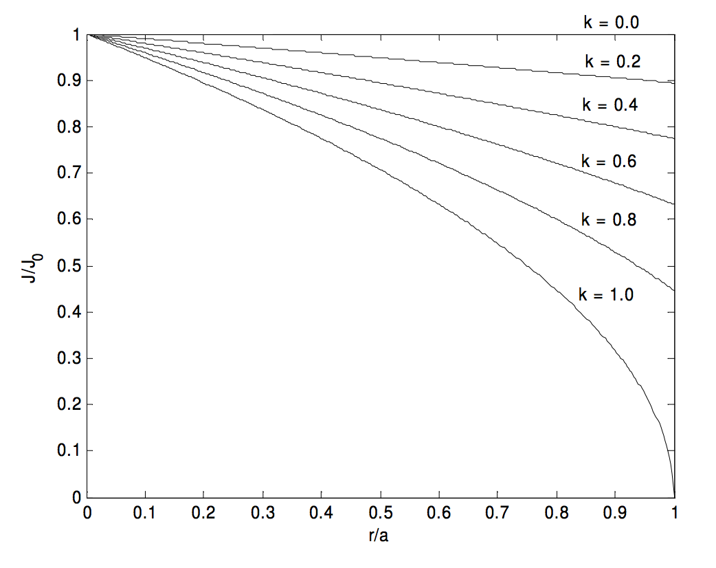
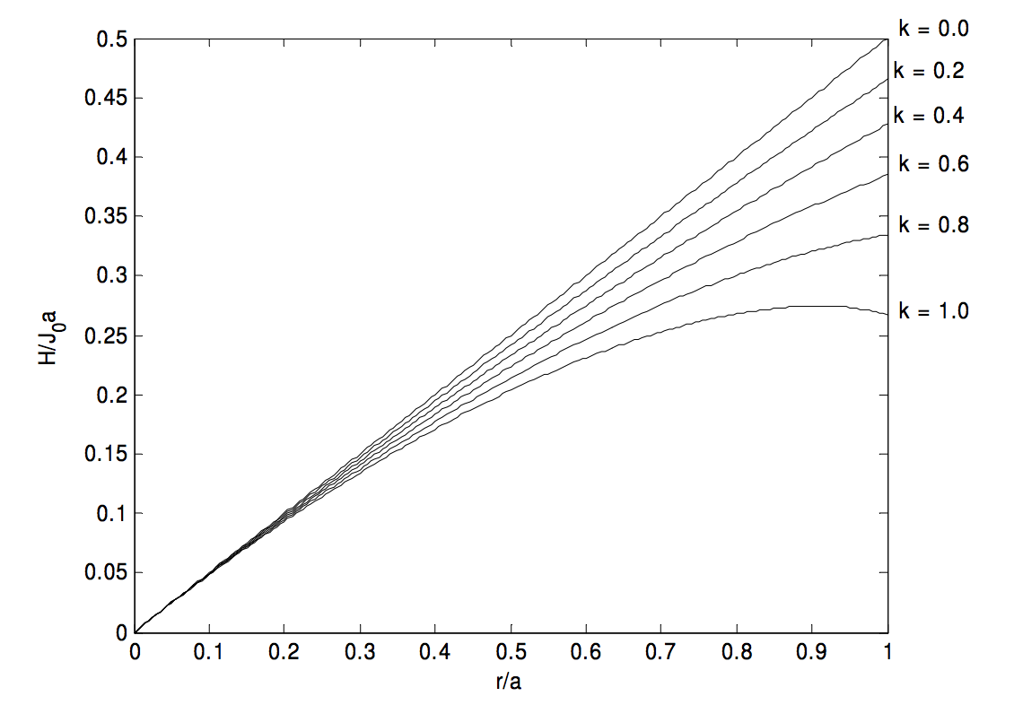
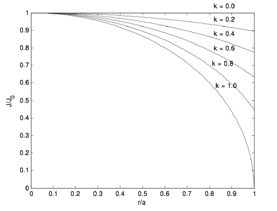
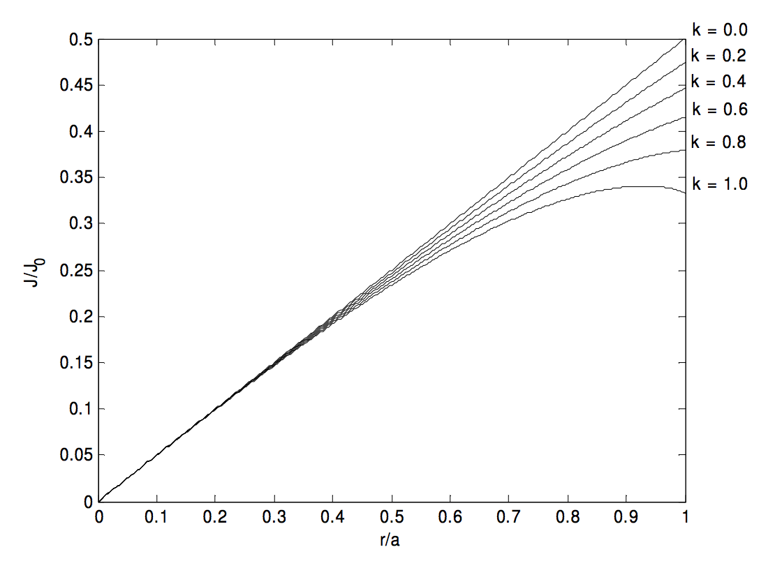
1:J(r)=J0(1−kra); 2:J(r)=J0(1−kr2a2); 3:J(r)=J0√1−kra; 4:J(r)=J0√1−kr2a2.
The mean current density is ¯J=2a2∫a0rJ(r)dr, and the total current is πa2 times this.
The magnetic field is H(r)=1r∫r0xJ(x)dx.
Here are the results:
1. J=J0(1−kra),¯J=J0(1−2k3),H(r)=J0(r2−kr23a).
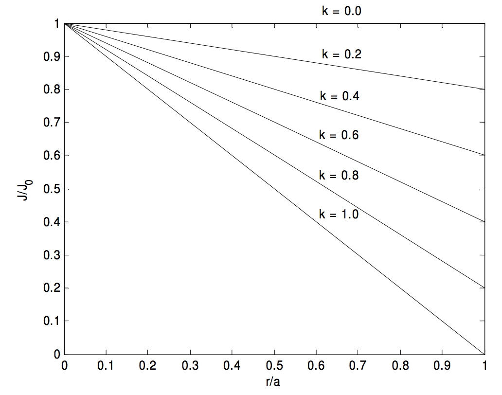
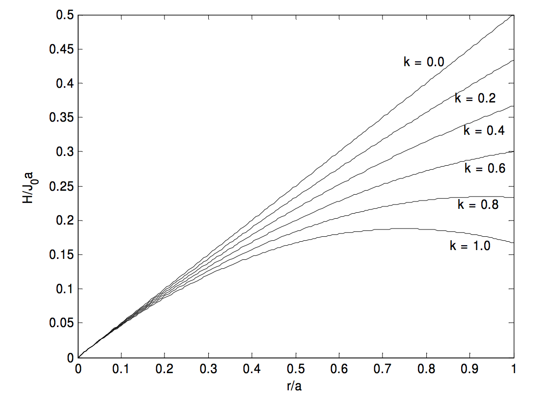
H reaches a maximum value of 3J0a16k at r=3a4k, but this maximum occurs inside the cylinder only if k>34.
2. J=J0(1−kr2a2),¯J=J0(1−12k),H(r)=J0(r2−kr34a2).
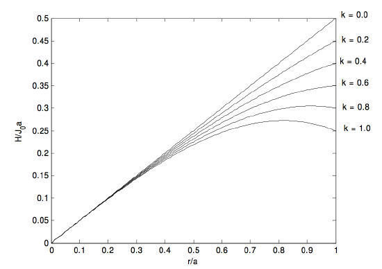
H reaches a maximum value of √227kJ0 at ra=√23k, but this maximum occurs inside the cylinder only if k>23.
3. J=J0√1−kra,¯J=J015k2[8−20(1−k)3/2+12(1−k)5/2],H(r)=2J0a215k2r[2−5(1−kra)3/2+3(1−kra)5/2].
I have not calculated explicit formulas for the positions and values of the maxima. A maximum occurs inside the cylinder if k>0.908901.
4. J=J0√1−kr2a2,¯J=2J03k[1−(1−k)3/2],H(r)=J0a23kr[1−(1−kr2a2)3/2].
A maximum occurs inside the cylinder if k>0.866025.
In all of these cases, the condition that there shall be no maximum H inside the cylinder – that is, between r=0 and r=a - is that J(a)¯J>12. I believe this to be true for any axially symmetric current density distribution, though I have not proved it. I expect that a fairly simple proof could be found by someone interested.
Additional current density distributions that readers might like to investigate are
J=J01+x/aJ=J01+x2/a2J=J0√1+x/a
J=J0√1+x2/a2J=J0e−x/aJ=J0e−x2/a2