2.2: Electromagnetic Waves in the Time Domain

Perhaps the greatest triumph of Maxwell’s equations was their ability to predict in a simple way the existence and velocity of electromagnetic waves based on simple laboratory measurements of the permittivity and permeability of vacuum. In vacuum the charge density \(\rho=\overline{\mathrm{J}}=0\), and so Maxwell’s equations become:

\[\nabla \times \overline{\mathrm{E}}=-\mu_{\mathrm{o}} \frac{\partial \overline{\mathrm{H}}}{\partial \mathrm{t}} \quad \quad \quad \quad \quad(\text { Faraday's law in vacuum })\]

\[\nabla \times \overline{\mathrm{H}}=\varepsilon_{\mathrm{o}} \frac{\partial \overline{\mathrm{E}}}{\partial \mathrm{t}} \quad \quad\quad\quad\quad(\text { Ampere's law in vacuum })\]

\[\nabla \cdot \overline{\mathrm{E}}=0\quad\quad\quad\quad\quad\text{(Gauss’s law in vacuum) } \]

\[\nabla \cdot \overline{\mathrm{H}}=0\quad\quad\quad\quad\quad\text{(Gauss’s law in vacuum) } \]

We can eliminate \(\overline H \) from these equations by computing the curl of Faraday’s law, which introduces \(\nabla \times \overline{\mathrm{H}}\) on its right-hand side so Ampere’s law can be substituted:

\[\nabla \times(\nabla \times \overline{\mathrm{E}})=-\mu_{\mathrm{o}} \frac{\partial(\nabla \times \overline{\mathrm{H}})}{\partial \mathrm{t}}=-\mu_{\mathrm{o}} \varepsilon_{\mathrm{o}} \frac{\partial \overline{\mathrm{E}}^{2}}{\partial \mathrm{t}^{2}}\]

Using the well known overlinetor identity (see Appendix D):

\[\nabla \times(\nabla \times \overline{A})=\nabla(\nabla \bullet \overline{A})-\nabla^{2} \overline{A} \quad\quad\quad\quad\quad( \text {"well-known overlinetor identity"})\]

and then using (2.2.3) to eliminate \( \nabla \bullet \overline{\mathrm{E}}\), (2.2.5) becomes the electromagnetic wave equation, often called the Helmholtz wave equation:

\[\nabla^{2} \overline{E}-\mu_{0} \varepsilon_{0} \frac{\partial^{2} \overline{E}}{\partial t^{2}}=0 \quad\quad\quad\quad\quad \text{(Helmholtz wave equation)} \]

where:

\[ \nabla^{2} \overline{E} \equiv\left(\frac{\partial^{2}}{\partial x^{2}}+\frac{\partial^{2}}{\partial y^{2}}+\frac{\partial^{2}}{\partial z^{2}}\right)\left(\hat{x} E_{x}+\hat{y} E_{y}+\hat{z} E_{z}\right)\]

The solutions to this wave equation (2.2.7) are any fields \(\overline{\mathrm{E}}(\overline{\mathrm{r}}, \mathrm{t})\) for which the second spatial derivative \(\left(\nabla^{2} \overline{E}\right) \) equals a constant times the second time derivative \(\left(\partial^{2} \overline{\mathrm{E}} / \partial \mathrm{t}^{2}\right)\). The position overlinetor \(\overline{\mathrm{r}} \equiv \hat{x} \mathrm{x}+\hat{y} \mathrm{y}+\hat{z} \mathrm{z} \). The wave equation is therefore satisfied by any arbitrary \(\overline{\mathrm{E}}(\overline{\mathrm{r}}, \mathrm{t}) \) having identical dependence on space and time within a constant multiplier. For example, arbitrary functions of the arguments (z - ct), (z + ct), or (t ± z/c) have such an identical dependence and are among the valid solutions to (2.2.7), where c is some constant to be determined. One such solution is:

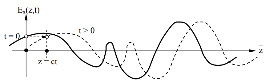
\[\overline{\mathrm{E}}(\overline{\mathrm{r}}, \mathrm{t})=\overline{\mathrm{E}}(\mathrm{z}-\mathrm{ct})=\hat{x} \mathrm{E}_{\mathrm{x}}(\mathrm{z}-\mathrm{ct}) \]

where the arbitrary function E_x(z - ct) might be that illustrated in Figure 2.2.1 at time t = 0 and again at some later time t. Note that as time advances within the argument (z - ct), z must advance with ct in order for that argument, or \(\overline E\) at any point of interest on the waveform, to remain constant.

Figure \(\PageIndex{1}\): Arbitrary electromagnetic wave propagating in the +z direction.

We can test this candidate solution (2.2.9) by substituting it into the wave equation (2.2.7), yielding:

\[ \begin{align}
\nabla^{2} \overline{E}(z-c t) &=\frac{\partial^{2}[\overline{E}(z-c t)]}{\partial z^{2}} \equiv \overline{E}^{\prime \prime}(z-c t) \\
&=\mu_{0} \varepsilon_{0} \frac{\partial^{2}[\overline{E}(z-c t)]}{\partial t^{2}}=\mu_{0} \varepsilon_{0}(-c)^{2} \overline{E}^{\prime \prime}(z-c t) \nonumber
\end{align}\]

where we define \( \overline{\mathrm{A}}^{\prime}(q)\) as the first derivative of \( \overline{\mathrm{A}}\) with respect to its argument q and \(\overline{\mathrm{A}}^{\prime \prime}(q) \) as its second derivative. Equation (2.2.10) is satisfied if:

\[ \mathrm{c}=\frac{1}{\sqrt{\mu_{0} \varepsilon_{0}}} \quad[\mathrm{m} / \mathrm{s}]\]

where we define c as the velocity of light in vacuum:

\[\mathrm{c}=2.998 \times 10^{8}\left[\mathrm{m} \mathrm{s}^{-1}\right] \quad \quad \quad \quad \quad \text{(velocity of light)} \]

Figure 2.2.1 illustrates how an arbitrary \( \overline{\mathrm{E}}(\mathrm{z}, \mathrm{t})\) can propagate by translating at velocity c. However, some caution is warranted when \(\overline{\mathrm{E}}(\mathrm{z}, \mathrm{t})\) is defined. Although our trial solution (2.2.9) satisfies the wave equation (2.2.7), it may not satisfy Gauss’s laws. For example, consider the case where:

\[\overline{\mathrm{E}}(\mathrm{z}, \mathrm{t})=\hat{z} \mathrm{E}_{\mathrm{z}}(\mathrm{z}-\mathrm{ct}) \]

Then Gauss’s law \(\nabla \bullet \overline{\mathrm{E}}=0 \) is not satisfied:

\[\nabla \bullet \overline{\mathrm{E}}=\frac{\partial \overline{\mathrm{E}}_{\mathrm{Z}}}{\partial \mathrm{Z}} \neq 0 \text { for arbitrary } \overline{\mathrm{E}}(\mathrm{z}) \]

In contrast, if \(\overline{\mathrm{E}}(\mathrm{z}, \mathrm{t}) \) is oriented perpendicular to the direction of propagation (in the \(\hat{x} \) and/or \(\hat{y}\) directions for z-directed propagation), then all Maxwell’s equations are satisfied and the solution is valid. In the case \(\overline{\mathrm{E}}(\mathrm{z}, \mathrm{t})=\hat{y} \mathrm{E}_{\mathrm{y}}(\mathrm{z}-\mathrm{ct}) \), independent of x and y, we have a uniform plane wave because the fields are uniform with respect to two of the coordinates (x,y) so that \( \partial \overline{\mathrm{E}} / \partial \mathrm{x}=\partial \overline{\mathrm{E}} / \partial \mathrm{y}=0\). Since this electric field is in the y direction, it is said to be y-polarized; by convention, polarization of a wave refers to the direction of its electric overlinetor. Polarization is discussed further in Section 2.3.4.

Knowing \(\overline{\mathrm{E}}(\mathrm{z}, \mathrm{t})=\hat{y} \mathrm{E}_{\mathrm{y}}(\mathrm{z}-\mathrm{ct})\) for this example, we can now find \( \overline{\mathrm{H}}(\mathrm{z}, \mathrm{t})\) using Faraday’s law (2.2.1):

\[\frac{\partial \overline{\mathrm{H}}}{\partial \mathrm{t}}=-\frac{(\nabla \times \overline{\mathrm{E}})}{\mu_{\mathrm{o}}} \]

We can evaluate the curl of \(\overline E\) using (2.1.4) and knowing \( \mathrm{E}_{\mathrm{x}}=\mathrm{E}_{\mathrm{z}}=\frac{\partial}{\partial \mathrm{x}}=\frac{\partial}{\partial \mathrm{y}}=0\):

\[\nabla \times \overline{\mathrm{E}}=\hat{x}\left(\frac{\partial \mathrm{E}_{\mathrm{z}}}{\partial \mathrm{y}}-\frac{\partial \mathrm{E}_{\mathrm{y}}}{\partial \mathrm{z}}\right)+\hat{y}\left(\frac{\partial \mathrm{E}_{\mathrm{x}}}{\partial \mathrm{z}}-\frac{\partial \mathrm{E}_{\mathrm{z}}}{\partial \mathrm{x}}\right)+\hat{z}\left(\frac{\partial \mathrm{E}_{\mathrm{y}}}{\partial \mathrm{x}}-\frac{\partial \mathrm{E}_{\mathrm{x}}}{\partial \mathrm{y}}\right)=-\hat{x} \frac{\partial \mathrm{E}_{\mathrm{y}}}{\partial \mathrm{z}} \]

Then, by integrating (2.2.15) over time it becomes:

\[ \begin{align}
\overline{\mathrm{H}}(\mathrm{z}, \mathrm{t}) &=-\int_{-\infty}^{\mathrm{t}} \frac{(\nabla \times \overline{\mathrm{E}})}{\mu_{\mathrm{o}}} \mathrm{dt}=\hat{x} \frac{1}{\mu_{\mathrm{o}}} \int_{-\infty}^{\mathrm{t}} \frac{\partial \mathrm{E}_{\mathrm{y}}(\mathrm{z}-\mathrm{ct})}{\partial \mathrm{z}} \mathrm{dt} \\
&=-\hat{x} \frac{1}{\mathrm{c} \mu_{\mathrm{o}}} \mathrm{E}_{\mathrm{y}}(\mathrm{z}-\mathrm{ct})=-\hat{x} \sqrt{\frac{\varepsilon_{\mathrm{o}}}{\mu_{\mathrm{o}}}} \mathrm{E}_{\mathrm{y}}(\mathrm{z}-\mathrm{ct})\nonumber
\end{align}\]

\[\overline{\mathrm{H}}(\mathrm{z}, \mathrm{t})=\sqrt{\frac{\varepsilon_{\mathrm{O}}}{\mu_{\mathrm{o}}}} \hat{z} \times \overline{\mathrm{E}}(\mathrm{z}, \mathrm{t})=\hat{z} \times \frac{\overline{\mathrm{E}}(\mathrm{z}, \mathrm{t})}{\eta_{\mathrm{o}}} \]

where we used the velocity of light \(\mathrm{c}=1 / \sqrt{\varepsilon_{\mathrm{o}} \mu_{\mathrm{o}}} \), and defined \(\eta_{\mathrm{o}}=\sqrt{\mu_{\mathrm{o}} / \varepsilon_{\mathrm{o}}} \).

Thus \(\overline E\) and \(\overline H\) in a uniform plane wave are very simply related. Their directions are orthogonal to each other and to the direction of propagation, and the magnitude of the electric field is \(\left(\mu_{0} / \varepsilon_{0}\right)^{0.5} \) times that of the magnetic field; this factor\(\eta_{\mathrm{o}}=\sqrt{\mu_{\mathrm{o}} / \varepsilon_{\mathrm{o}}} \) is known as the characteristic impedance of free space and equals ~377 ohms. That is, for a single uniform plane wave in free space,

\[ |\overline{\mathrm{E}} /| \overline{\mathrm{H}} |=\eta_{\mathrm{o}}=\sqrt{\mu_{\mathrm{o}} / \varepsilon_{\mathrm{o}}} \cong 377 \ [\mathrm{ohms}]\]

Electromagnetic waves can propagate in any arbitrary direction in space with arbitrary time behavior. That is, we are free to define \(\hat{x}\), \(\hat{y}\), and \(\hat{z}\) in this example as being in any three orthogonal directions in space. Because Maxwell’s equations are linear in field strength, superposition applies and any number of plane waves propagating in arbitrary directions with arbitrary polarizations can be superimposed to yield valid electromagnetic solutions. Exactly which superposition is the valid solution in any particular case depends on the boundary conditions and the initial conditions for that case, as discussed later in Chapter 9 for a variety of geometries.

Example \(\PageIndex{A}\)

Show that \( \overline{\mathrm{E}}=\hat{y} \mathrm{E}_{\mathrm{o}}(\mathrm{t}+\mathrm{z} / \mathrm{c})\) satisfies the wave equation (2.2.7). In which direction does this wave propagate?

Solution

\( \left(\nabla^{2}-\frac{\partial^{2}}{c^{2} \partial t^{2}}\right) \overline{E}=\hat{y} \frac{1}{c^{2}}\left[E_{0}^{\prime \prime}(t+z / c)-E_{0}^{\prime \prime}(t+z / c)\right]=0\); Q.E.D⁴ .

Since the argument remains constant as t increases only if z/c decreases correspondingly, the wave is propagating in the -z direction.

⁴ Q.E.D. is the abbreviation for the Latin phrase “quod erat demonstratum” or “that which was to be demonstrated.”