2.6: Boundary conditions for electromagnetic fields

Introduction

Maxwell’s equations characterize macroscopic matter by means of its permittivity ε, permeability μ, and conductivity σ, where these properties are usually represented by scalars and can vary among media. Section 2.5 discussed media for which ε, μ, and σ are represented by matrices, complex quantities, or other means. This Section 2.6 discusses how Maxwell’s equations strongly constrain the behavior of electromagnetic fields at boundaries between two media having different properties, where these constraint equations are called boundary conditions. Section 2.6.2 discusses the boundary conditions governing field components perpendicular to the boundary, and Section 2.6.3 discusses the conditions governing the parallel field components. Section 2.6.4 then treats the special case of fields adjacent to perfect conductors.

One result of these boundary conditions is that waves at boundaries are generally partially transmitted and partially reflected with directions and amplitudes that depend on the two media and the incident angles and polarizations. Static fields also generally have different amplitudes and directions on the two sides of a boundary. Some boundaries in both static and dynamic situations also possess surface charge or carry surface currents that further affect the adjacent fields.

The boundary conditions governing the perpendicular components of \(\overline E\) and \(\overline H\) follow from the integral forms of Gauss’s laws:

\[\oiint_{\mathrm{S}}(\overline{\mathrm{D}} \bullet \hat{n}) \mathrm{d} \mathrm{a}=\int \int \int_{\mathrm{V}} \rho \mathrm{d} \mathrm{v} \quad\quad\quad\quad\quad(\text {Gauss 's Law for } \overline{\mathrm{D}})\]

\[\oiint_{S}(\overline{\mathrm{B}} \bullet \hat{n}) \mathrm{d} \mathrm{a}=0 \quad\quad\quad\quad\quad(\text {Gauss 's Law for }\overline{\mathrm{B}})\]

We may integrate these equations over the surface S and volume V of the thin infinitesimal pillbox illustrated in Figure 2.6.1. The pillbox is parallel to the surface and straddles it, half being on each side of the boundary. The thickness δ of the pillbox approaches zero faster than does its surface area S, where S is approximately twice the area A of the top surface of the box.

Figure \(\PageIndex{1}\): Elemental volume for deriving boundary conditions for perpendicular field components.

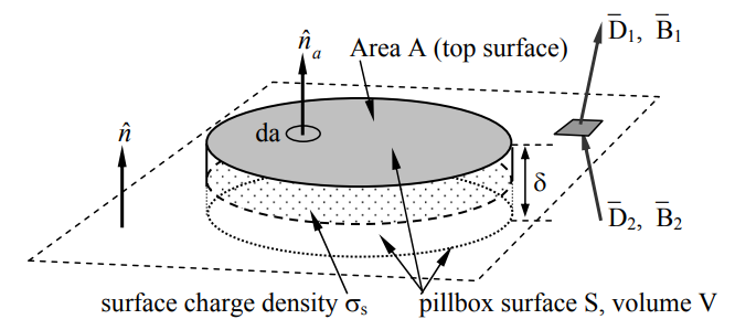
Beginning with the boundary condition for the perpendicular component D_⊥, we integrate Gauss’s law (2.6.1) over the pillbox to obtain:

\[\oiint_{\mathrm{S}}\left(\overline{\mathrm{D}} \bullet \hat{n}_{a}\right) \mathrm{da} \cong\left(\mathrm{D}_{1 \perp}-\mathrm{D}_{2 \perp}\right) \mathrm{A}=\int \int \int_{\mathrm{V}} \rho \mathrm{d} \mathrm{v}=\rho_{\mathrm{s}} \mathrm{A}\]

where ρ_s is the surface charge density [Coulombs m^-2]. The subscript s for surface charge ρ_s distinguishes it from the volume charge density ρ [C m^-3]. The pillbox is so thin (δ → 0) that: 1) the contribution to the surface integral of the sides of the pillbox vanishes in comparison to the rest of the integral, and 2) only a surface charge q can be contained within it, where ρ_s = q/A = lim ρδ as the charge density ρ → ∞ and δ → 0. Thus (2.6.3) becomes D_1⊥ - D_2⊥ = ρ_s, which can be written as:

\[\left.\hat{n} \bullet\left(\overline{\mathrm{D}}_{1}-\overline{\mathrm{D}}_{2}\right)=\rho_{\mathrm{s}} \quad\quad\quad\quad\quad \text { (boundary condition for } \overline{\mathrm{D}}_{\perp}\right)\]

where \(\hat{n}\) is the unit overlinetor normal to the boundary and points into medium 1. Thus the perpendicular component of the electric displacement overlinetor \(\overline D\) changes value at a boundary in accord with the surface charge density ρ_s.

Because Gauss’s laws are the same for electric and magnetic fields, except that there are no magnetic charges, the same analysis for the magnetic flux density \(\overline B\) in (2.6.2) yields a similar boundary condition:

\[\left.\hat{n} \bullet\left(\overline{\mathrm{B}}_{1}-\overline{\mathrm{B}}_{2}\right)=0 \quad\quad\quad\quad\quad \text { (boundary condition for } \overline{\mathrm{B}}_{\perp}\right)\]

Thus the perpendicular component of \(\overline B\) must be continuous across any boundary.

Boundary conditions for parallel field components

The boundary conditions governing the parallel components of \(overline E\) and \(\overline H\) follow from Faraday’s and Ampere’s laws:

\[\oint_{C} \overline{E} \bullet d \overline{s}=-\frac{\partial}{\partial t} \int \int_{A} \overline{B} \bullet \hat{n} d a \quad\quad\quad\quad\quad(\text {Faraday's Law})\]

\[\oint_{\mathrm{C}} \overline{\mathrm{H}} \bullet \mathrm{d} \overline{\mathrm{s}}=\int \int_{\mathrm{A}}\left[\overline{\mathrm{J}}+\frac{\partial \overline{\mathrm{D}}}{\partial \mathrm{t}}\right] \bullet \hat{n} \mathrm{da} \quad \quad\quad\quad\quad(\text {Ampere's } L a w)\]

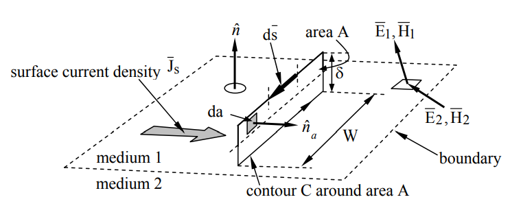
We can integrate these equations around the elongated rectangular contour C that straddles the boundary and has infinitesimal area A, as illustrated in Figure 2.6.2. We assume the total height δ of the rectangle is much less than its length W, and circle C in a right-hand sense relative to the surface normal \(\hat{n}_{\mathrm{a}}\).

Figure \(\PageIndex{2}\): Elemental contour for deriving boundary conditions for parallel field components.

Beginning with Faraday’s law, (2.6.6), we find:

\[\oint_{\mathrm{C}} \overline{\mathrm{E}} \bullet \mathrm{d} \overline{\mathrm{s}} \cong\left(\overline{\mathrm{E}}_{1 / /}-\overline{\mathrm{E}}_{2 / /}\right) \mathrm{W}=-\frac{\partial}{\partial \mathrm{t}} \int \int_{\mathrm{A}} \overline{\mathrm{B}} \bullet \hat{n}_{a} \mathrm{da} \rightarrow 0\]

where the integral of \(\overline B\) over area A approaches zero in the limit where δ approaches zero too; there can be no impulses in \(\overline B\). Since W ≠ 0, it follows from (2.6.8) that E_1// - E_2// = 0, or more generally:

\[\left.\hat{n} \times\left(\overline{\mathrm{E}}_{1}-\overline{\mathrm{E}}_{2}\right)=0 \quad \quad \quad \quad \quad \text { (boundary condition for } \overline{\mathrm{E}}_{/ /}\right)\]

Thus the parallel component of \(\overline E\) must be continuous across any boundary.

A similar integration of Ampere’s law, (2.6.7), under the assumption that the contour C is chosen to lie in a plane perpendicular to the surface current \(\overline{J}_{S}\) and is traversed in the right-hand sense, yields:

\[\begin{align} \oint_{\mathrm{C}} \overline{\mathrm{H}} \bullet \mathrm{d} \overline{\mathrm{s}} &=\left(\overline{\mathrm{H}}_{1 / /}-\overline{\mathrm{H}}_{2 / /}\right) \mathrm{W} \\ &=\int \int_{\mathrm{A}}\left[\overline{\mathrm{J}}+\frac{\partial \overline{\mathrm{D}}}{\partial \mathrm{t}}\right] \bullet \hat{n} \mathrm{da} \Rightarrow \int \int_{\mathrm{A}} \overline{\mathrm{J}} \bullet \hat{n}_{a} \mathrm{d} \mathrm{a}=\overline{\mathrm{J}}_{\mathrm{S}} \mathrm{W} \nonumber \end{align}\]

where we note that the area integral of \(\partial \overline{\mathrm{D}} / \partial t\) approaches zero as δ → 0, but not the integral over the surface current \(\overline{\mathrm{J}}_{\mathrm{s}}\), which occupies a surface layer thin compared to δ. Thus \(\overline{\mathrm{H}}_{1 / /}-\overline{\mathrm{H}}_{2 / /}=\overline{\mathrm{J}}_{\mathrm{S}}\), or more generally:

\[\left.\hat{n} \times\left(\overline{\mathrm{H}}_{1}-\overline{\mathrm{H}}_{2}\right)=\overline{\mathrm{J}}_{\mathrm{s}} \quad \quad \quad \quad \quad \text { (boundary condition for } \overline{\mathrm{H}}_{ //}\right)\]

where \(\hat{n}\) is defined as pointing from medium 2 into medium 1. If the medium is nonconducting, \( \overline{\mathrm{J}}_{\mathrm{s}}=0\).

A simple static example illustrates how these boundary conditions generally result in fields on two sides of a boundary pointing in different directions. Consider the magnetic fields \(\overline{\mathrm{H}}_{1} \) and \(\overline{\mathrm{H}}_{2} \) illustrated in Figure 2.6.3, where \( \mu_{2} \neq \mu_{1}\), and both media are insulators so the surface current must be zero. If we are given \( \overline{\mathrm{H}}_{1}\), then the magnitude and angle of \( \overline{\mathrm{H}}_{2}\) are determined because \( \overline{\mathrm{H}}_{/ /}\) and \( \overline{\mathrm{B}}_{\perp}\) are continuous across the boundary, where \(\overline{\mathrm{B}}_{\mathrm{i}}=\mu_{\mathrm{i}} \overline{\mathrm{H}}_{\mathrm{i}} \). More specifically, \( \overline{\mathrm{H}}_{2 / /}=\overline{\mathrm{H}}_{1 / /}\), and:

\[ \mathrm{H}_{2 \perp}=\mathrm{B}_{2 \perp} / \mu_{2}=\mathrm{B}_{1 \perp} / \mu_{2}=\mu_{1} \mathrm{H}_{1 \perp} / \mu_{2}\]

Figure \(\PageIndex{3}\): Static magnetic field directions at a boundary.

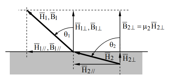
It follows that:

\[\theta_{2}=\tan ^{-1}\left(\left|\overline{\mathrm{H}}_{2 / /}\right| / \mathrm{H}_{2 \perp}\right)=\tan ^{-1}\left(\mu_{2}\left|\overline{\mathrm{H}}_{1 / /}\right| / \mu_{1} \mathrm{H}_{1 \perp}\right)=\tan ^{-1}\left[\left(\mu_{2} / \mu_{1}\right) \tan \theta_{1}\right]\]

Thus θ₂ approaches 90 degrees when μ₂ >> μ₁, almost regardless of θ₁, so the magnetic flux inside high permeability materials is nearly parallel to the walls and trapped inside, even when the field orientation outside the medium is nearly perpendicular to the interface. The flux escapes high-μ material best when θ₁ ≅ 90°. This phenomenon is critical to the design of motors or other systems incorporating iron or nickel.

If a static surface current \(\overline{\mathrm{J}}_{\mathrm{S}}\) flows at the boundary, then the relations between \(\overline{\mathrm{B}}_{1}\) and \(\overline{\mathrm{B}}_{2}\) are altered along with those for \(\overline{\mathrm{H}}_{1}\) and \(\overline{\mathrm{H}}_{2}\). Similar considerations and methods apply to static electric fields at a boundary, where any static surface charge on the boundary alters the relationship between \(\overline{\mathrm{D}}_{1}\) and \(\overline{\mathrm{D}}_{2}\). Surface currents normally arise only in non-static or “dynamic” cases.

Example \(\PageIndex{A}\)

Two insulating planar dielectric slabs having ε₁ and ε₂ are bonded together. Slab 1 has \(\overline{\mathrm{E}}_{1}\) at angle θ₁ to the surface normal. What are \(\overline{\mathrm{E}}_{2}\) and θ₂ if we assume the surface charge at the boundary ρ_s = 0? What are the components of \(\overline{\mathrm{E}}_{2}\)\) if ρs ≠ 0?

Solution

\(\overline{\mathrm{E}} / /\) is continuous across any boundary, and if _ρs = 0, then \(\overline{\mathrm{D}}_{\perp}=\varepsilon_{\mathrm{i}} \overline{\mathrm{E}}_{\perp}\) is continuous too, which implies \(\overline{\mathrm{E}}_{2 \perp}=\left(\varepsilon_{1} / \varepsilon_{2}\right) \overline{\mathrm{E}}_{1 \perp}\). Also, \(\theta_{1}=\tan ^{-1}\left(\mathrm{E}_{/ /} / \mathrm{E}_{1 \perp}\right)\), and \(\theta_{2}=\tan ^{-1}\left(\mathrm{E}_{/ /} / \mathrm{E}_{2 \perp}\right)\). It follows that \(\theta_{2}=\tan ^{-1}\left[\left(\varepsilon_{2} / \varepsilon_{1}\right) \tan \theta_{1}\right]\). If ρ_s ≠ 0 then \(\overline{\mathrm{E}}_{/ /}\) is unaffected and \(\overline{\mathrm{D}}_{2 \perp}=\overline{\mathrm{D}}_{1 \perp}+\hat{n} \rho_{\mathrm{s}}\) so that \(\overline{\mathrm{E}}_{2 \perp}=\overline{\mathrm{D}}_{2 \perp} / \varepsilon_{2}=\left(\varepsilon_{1} / \varepsilon_{2}\right) \overline{\mathrm{E}}_{1 \perp}+\hat{n} \rho_{\mathrm{s}} / \varepsilon_{2}\).

Boundary conditions adjacent to perfect conductors

The four boundary conditions (2.6.4), (2.6.5), (2.6.9), and (2.6.11) are simplified when one medium is a perfect conductor (σ = ∞) because electric and magnetic fields must be zero inside it. The electric field is zero because otherwise it would produce enormous \(\overline{\mathrm{J}}=\sigma \overline{\mathrm{E}}\) so as to redistribute the charges and to neutralize that \(\overline E\) almost instantly, with a time constant \(\tau\) =εσ seconds, as shown in Equation (4.3.3).

It can also be easily shown that \(\overline B\) is zero inside perfect conductors. Faraday’s law says \(\nabla \times \overline{\mathrm{E}}=-\partial \overline{\mathrm{B}} / \partial \mathrm{t}\) so if \(\overline E\)= 0 , then \(\partial \overline{\mathrm{B}} / \partial \mathrm{t}=0\). If the perfect conductor were created in the absence of \(\overline B\) then \(\overline B\) would always remain zero inside. It has further been observed that when certain special materials become superconducting at low temperatures, as discussed in Section 2.5.2, any pre-existing \(\overline B\) is thrust outside.

The boundary conditions for perfect conductors are also relevant for normal conductors because most metals have sufficient conductivity σ to enable \(\overline J\) and ρ_s to cancel the incident electric field, although not instantly. As discussed in Section 4.3.1, this relaxation process by which charges move to cancel \(\overline E\) is sufficiently fast for most metallic conductors that they largely obey the perfect-conductor boundary conditions for most wavelengths of interest, from DC to beyond the infrared region. This relaxation time constant is \(\tau\) = ε/σ seconds. One consequence of finite conductivity is that any surface current penetrates metals to some depth \(\delta=\sqrt{2 / \omega \mu \sigma}\), called the skin depth, as discussed in Section 9.2. At sufficiently low frequencies, even sea water with its limited conductivity largely obeys the perfect-conductor boundary condition.

The four boundary conditions for fields adjacent to perfect conductors are presented below together with the more general boundary condition from which they follow when all fields in medium 2 are zero:

\[ \hat{n} \bullet \overline{\mathrm{B}}=0 \quad\quad\quad\quad\quad\left[\text { from } \hat{n} \bullet\left(\overline{\mathrm{B}}_{1}-\overline{\mathrm{B}}_{2}\right)=0\right]\]

\[\hat{n} \bullet \overline{\mathrm{D}}=\rho_{\mathrm{s}} \quad\quad\quad\quad\quad\left[\text { from } \hat{n} \bullet\left(\overline{\mathrm{D}}_{1}-\overline{\mathrm{D}}_{2}\right)=\rho_{\mathrm{s}}\right] \]

\[ \hat{n} \times \overline{\mathrm{E}}=0 \quad\quad\quad\quad\quad\left[\text { from } \hat{n} \times\left(\overline{\mathrm{E}}_{1}-\overline{\mathrm{E}}_{2}\right)=0\right]\]

\[ \hat{n} \times \overline{\mathrm{H}}=\overline{\mathrm{J}}_{\mathrm{S}} \quad\quad\quad\quad\quad\left[\text { from } \hat{n} \times\left(\overline{\mathrm{H}}_{1}-\overline{\mathrm{H}}_{2}\right)=\overline{\mathrm{J}}_{\mathrm{S}}\right]\]

These four boundary conditions state that magnetic fields can only be parallel to perfect conductors, while electric fields can only be perpendicular. Moreover, the magnetic fields are always associated with surface currents flowing in an orthogonal direction; these currents have a numerical value equal to \(\overline H\). The perpendicular electric fields are always associated with a surface charge ρs numerically equal to \(\overline D\) ; the sign of σ is positive when \(\overline D\) points away from the conductor.

Example \(\PageIndex{B}\)

What boundary conditions apply when μ→∞, σ = 0, and ε = ε_o?

Solution

Inside this medium \(\overline H\) = 0 and \(\overline J\) = 0 because otherwise infinite energy densities, \(\mu|\mathrm{H}|^{2} / 2\), are required; static \(\overline E\) and \(\overline B\) are unconstrained, however. Since \(\nabla \times \overline{\mathrm{H}}=0=\overline{\mathrm{J}}+\partial \overline{\mathrm{D}} / \partial \mathrm{t}\) inside, dynamic \(\overline E\) and \(\overline D\) = 0 there too. Since \(\overline{\mathrm{H}}_{/ /}\) and \(\overline{\mathrm{B}}_{\perp}\) are continuous across the boundary, \(\overline{\mathrm{H}}_{/ /}=0\) and \(\overline{\mathrm{H}}_{\perp}\) can be anything at the boundary. Since \(\overline{\mathrm{E}}_{/ /}\) and \(\overline{\mathrm{D}}_{\perp}\) are continuous (let’s assume ρ_s = 0 if \(\overline J\) = 0 ), static \(\overline E\) and \(\overline D\) are unconstrained at the boundary while dynamic \(\overline{\mathrm{E}}=\overline{\mathrm{D}}=0\) there because there is no dynamic electric field inside and no dynamic surface charge. Since only \(\overline{\mathrm{H}}_{\perp} \neq 0\) at the boundary, this is non-physical and such media don’t exist. For example, there is no way to match boundary conditions for an incoming plane wave. This impasse would be avoided if σ ≠ 0, for then dynamic \(\overline{\mathrm{H}}_{/ /}\) and \(\overline{\mathrm{E}}_{\perp}\) could be non-zero.