
3.4: General circuits and solution methods


- Last updated
- Jun 7, 2025
- Save as PDF

( \newcommand{\kernel}{\mathrm{null}\,}\)
Kirchoff’s Laws
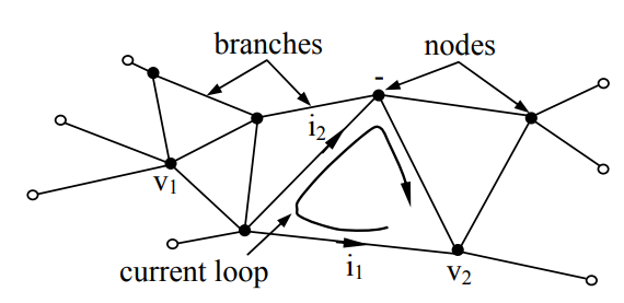
Circuits are generally composed of lumped elements or “branches” connected at nodes to form two- or three-dimensional structures, as suggested in Figure 3.4.1. They can be characterized by the voltages vi at each node or across each branch, or by the currents ij flowing in each branch or in a set of current loops. To determine the behavior of such circuits we develop simultaneous linear equations that must be satisfied by the unknown voltages and currents. Kirchoff’s laws generally provide these equations.
Although circuit analysis is often based in part on Kirchoff’s laws, these laws are imperfect due to electromagnetic effects. For example, Kirchoff’s voltage law (KVL) says that the voltage drops vi associated with each lumped element around any loop must sum to zero, i.e.:
∑ivi=0(Kirchoff’s voltage law [KVL])
which can be derived from the integral form of Faraday’s law:
∮C→E∙d→s=−(∂/∂t)⊂⊃∬A→B∙d→a
This integral of →E∙d→s across any branch yields the voltage across that branch. Therefore the sum of branch voltages around any closed contour is zero if the net magnetic flux through that contour is constant; this is the basic assumption of KVL.
KVL is clearly valid for any static circuit. However, any branch carrying time varying current will contribute time varying magnetic flux and therefore voltage to all adjacent loops plus others nearby. These voltage contributions are typically negligible because the currents and loop areas are small relative to the wavelengths of interest (λ = c/f) and the KVL approximation then applies. A standard approach to analyzing circuits that violate KVL is to determine the magnetic energy or inductance associated with any extraneous magnetic fields, and to model their effects in the circuit with a lumped parasitic inductance in each affected current loop.
The companion relation to KVL is Kirchoff’s current law (KCL), which says that the sum of the currents ij flowing into any node is zero:
∑jij=0(Kirchoff’s current law)
This follows from conservation of charge (2.4.19) when no charge storage on the nodes is allowed:
(∂/∂t)∫∫∫Vρdv=−⊂⊃∬A→J∙d→a(conservation of charge)
If no charge can be stored on the volume V of a node, then (∂/∂t)∫∫∫Vρdv=0, and there can be V no net current into that node.
For static problems, KCL is exact. However, the physical nodes and the wires connecting those nodes to lumped elements typically exhibit varying voltages and →D, and therefore have capacitance and the ability to store charge, violating KCL. If the frequency is sufficiently high that such parasitic capacitance at any node becomes important, that parasitic capacitance can be modeled as an additional lumped element attached to that node.
Solving circuit problems
To determine the behavior of any given linear lumped element circuit a set of simultaneous equations must be solved, where the number of equations must equal or exceed the number of unknowns. The unknowns are generally the voltages and currents on each branch; if there are b branches there are 2b unknowns.
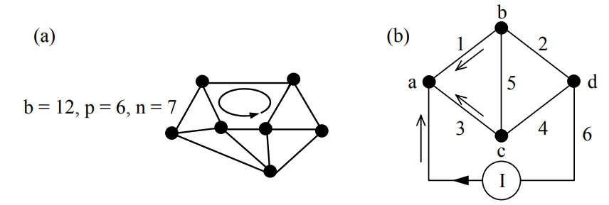
Figure 3.4.2(a) illustrates a simple circuit with b = 12 branches, p = 6 loops, and n = 7 nodes. A set of loop currents uniquely characterizes all currents if each loop circles only one “hole” in the topology and if no additional loops are added once every branch in the circuit is incorporated in at least one loop. Although other definitions for the loop currents can adequately characterize all branch currents, they are not explored here. Figure 3.4.2(b) illustrates a bridge circuit with b = 6, p = 3, and n = 4.
The simplest possible circuit has one node and one branch, as illustrated in Figure 3.4.3(a).
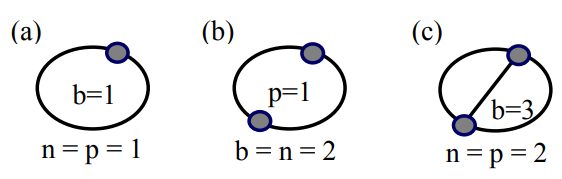
It is easy to see from the figure that the number b of branches in a circuit is:
b=n+p−1
As we add either nodes or branches to the illustrated circuit in any sequence and with any placement, Equation (3.4.5) is always obeyed. If we add voltage or current sources to the circuit, they too become branches.
The voltage and current for each branch are initially unknown and therefore any circuit has 2b unknowns. The number of equations is also b + (n – 1) + p = 2b, where the first b in this expression corresponds to the equations relating voltage to current in each branch, n-1 is the number of independent KCL equations, and p is the number of loops and KVL equations; (3.4.5) says (n – 1) + p = b. Therefore, since the numbers of unknowns and linear equations match, we may solve them. The equations are linear because Maxwell’s equations are linear for RLC circuits.
Often circuits are so complex that it is convenient for purposes of analysis to replace large sections of them with either a two-terminal Thevenin equivalent circuit or Norton equivalent circuit. This can be done only when that circuit is incrementally linear with respect to voltages imposed at its terminals. Thevenin equivalent circuits consist of a voltage source VTh(t) in series with a passive linear circuit characterized by its frequency-dependent impedance Z_(ω)=R+jX, while Norton equivalent circuits consist of a current source INo(t) in parallel with an impedance Z_(ω).
An important example of the utility of equivalent circuits is the problem of designing a matched load Z_L(ω)=RL(ω)+jXL(ω) that accepts the maximum amount of power available from a linear source circuit, and reflects none. The solution is simply to design the load so its impedance Z_L(ω) is the complex conjugate of the source impedance: Z_L(ω)=Z_∗(ω). For both Thevenin and Norton equivalent sources the reactance of the matched load cancels that of the source [XL(ω) = - X(ω)] and the two resistive parts are set equal, R = RL.
One proof that a matched load maximizes power transfer consists of computing the timeaverage power Pd dissipated in the load as a function of its impedance, equating to zero its derivative dPd/dω, and solving the resulting complex equation for RL and XL. We exclude the possibility of negative resistances here unless those of the load and source have the same sign; otherwise the transferred power can be infinite if RL = -R.
The bridge circuit of Figure 3.4.2(b) has five branches connecting four nodes in every possible way except one. Assume both parallel branches have 0.1-ohm and 0.2-ohm resistors in series, but in reverse order so that R1 = R4 = 0.1, and R2 = R3 = 0.2. What is the resistance R of the bridge circuit between nodes a and d if R5 = 0? What is R if R5 = ∞? What is R if R5 is 0.5 ohms?
Solution
When R5 = 0 then the node voltages vb = vc, so R1 and R3 are connected in parallel and have the equivalent resistance R13//. Kirchoff’s current law “KCL” (3.4.3) says the current flowing into node “a” is I = (va - vb)(R1-1 + R3-1). If Vab ≡ (va - vb), then Vab = IR13// and R13// = (R1-1 + R3-1)-1 = (10+5)-1 = 0.067Ω = R24//. These two circuits are in series so their resistances add: R = R13// + R24// ≅ 0.133 ohms. When R5 = ∞, R1 and R2 are in series with a total resistance R12s of 0.1 + 0.2 = 0.3Ω = R34s. These two resistances, R12s and R34s are in parallel, so R = (R12s-1 + R34s-1)-1 = 0.15Ω. When R5 is finite, then simultaneous equations must be solved. For example, the currents flowing into each of nodes a, b, and c sum to zero, yielding three simultaneous equations that can be solved for the vector →V=[va,vb,vc]; we define vd = 0. Thus
(va−vb)/R1+(va−vc)/R3=I=va(R−11+R−13)−vbR−11−vcR−13=15va−10vb−5vc.
KCL for nodes b and c similarly yield: -10va + 17vb - 2vc = 0, and -5va -2vb + 17vc = 0. If we define the current vector →I=[I,0,0], then these three equations can be written as a matrix equation:
→→G→v=→I, where →→G=[15−10−5−1017−2−5−217].
Since the desired circuit resistance between nodes a and d is R = va/I, we need only solve for va in terms of I, which follows from →v=→→G−1→I, provided the conductance matrix →→G is not singular (here it is not). Thus R = 0.146Ω, which is intermediate between the first two solutions, as it should be.