
4.3: Relaxation of Fields and Skin Depth


- Last updated
- Jun 7, 2025
- Save as PDF
( \newcommand{\kernel}{\mathrm{null}\,}\)
Relaxation of electric fields and charge in conducting media
lectric and magnetic fields established in conducting time-invariant homogeneous media tend to decay exponentially unless maintained. Under the quasistatic assumption all time variations are sufficiently slow that contributions to →E by ∂→B/∂t are negligible, which avoids wave-like behavior and simplifies the problem. This relaxation process is governed by the conservation-ofcharge relation (2.1.21), Gauss’s law (∇∙→D=ρ), and Ohm’s law (→J=σ→E):
∇∙→J+∂ρ/∂t=0=∇∙(σ→E)+(∂/∂t)(∇∙ε→E)=∇∙[(σ+ε∂/∂t)→E]=0
Since an arbitrary →E can be established by initial conditions, the general solution to (4.3.1) requires (σ+ε∂/∂t)∇∙→E=0, leading to the differential equation:
(∂/∂t+σ/ε)ρ=0
where ∇∙→E=ρ/ε. This has the solution that ρ(→r) relaxes exponentially with a charge relaxation time constant τ = ε/σ seconds:
ρ(ˉr)=ρ0(ˉr)e−σt/ε=ρ0(ˉr)e−t/π[−3]( charge relaxation )
It follows that an arbitrary initial electric field →E(→r) in a medium having uniform ε and σ will also decay exponentially with the same time constant ε/σ because Gauss’s law relates →E and ρ linearly:
∇∙→E=ρ(t)/ε
where . Therefore electric field relaxation is characterized by:
We should expect such exponential decay because any electric fields in a conductor will generate currents and therefore dissipate power proportional to J2 and E2 . But the stored electrical energy is also proportional to E2 , and power dissipation is the negative derivative of stored energy. That is, the energy decays at a rate proportional to its present value, which results in exponential decay. In copper τ = εo/σ ≅ 9×10-12/(5×107) ≅ 2×10-19 seconds, short compared to any delay of common interest. The special case of parallel-plate resistors and capacitors is discussed in Section 3.1.
What are the electric field relaxation time constants τ for sea water (ε ≅ 80εo, σ ≅ 4) and dry soil (ε ≅ 2εo, σ ≅ 10-5)? For what radio frequencies can they be considered good conductors?
Solution
Equation (4.3.5) yields τ = ε/σ ≅ (80×8.8×10-12)/4 ≅ 1.8×10⁻¹⁰ seconds for seawater, and (2×8.8×10-12)/10-5 ≅ 1.8×10⁻⁶ seconds for dry soil. So long as →E changes slowly with respect to τ, the medium has time to cancel →E; frequencies below ~5 GHz and ~500 kHz have this property for seawater and typical dry soil, respectively, which behave like good conductors at these lower frequencies. Moist soil behaves like a conductor up to ~5 MHz and higher.
Relaxation of magnetic fields in conducting media
Magnetic fields and their induced currents similarly decay exponentially in conducting media unless they are externally maintained; this decay process is often called magnetic diffusion or magnetic relaxation. We assume that the time variations are sufficiently slow that contributions to →H by ∂→D/∂t are negligible. In this limit Ampere’s law becomes:
∇×→H=→J=σ→E
∇×(∇×→H)=σ∇×→E=−σμ∂→H/∂t=−∇2→H+∇(∇∙→H)=−∇2→H
where Faraday’s law, the vector identity (2.2.6), and Gauss’s law (∇∙→B=0) were used.
The resulting differential equation:
σμ∂→H/∂t=∇2→H
has at least one simple solution:
→H(z,t)=ˆxHoe−t/τmcoskz
where we assumed an x-polarized z-varying sinusoid. Substituting (4.3.9) into (4.3.8) yields the desired time constant:
τm=μσ/k2=μσλ2/4π2[s] (magnetic relaxation time)
Thus the lifetime of magnetic field distributions in conducting media increases with permeability (energy storage density), conductivity (reducing dissipation for a given current), and the wavelength squared (λ = 2π/k).
Induced currents
Quasistatic magnetic fields induce electric fields by virtue of Faraday’s law: ∇×→E=−μ∂→H/∂t. In conductors these induced electric fields drive currents that obey Lenz’s law: “The direction of induced currents tends to oppose changes in magnetic flux.” Induced currents find wide application, for example, in: 1) heating, as in induction furnaces that melt metals, 2) mechanical actuation, as in induction motors and impulse generators, and 3) electromagnetic shielding. In some cases these induced currents are undesirable and are inhibited by subdividing the conductors into elements separated by thin insulating barriers. All these examples are discussed below.
First consider a simple conducting hollow cylinder of length W driven circumferentially by current Iou(t), as illustrated in Figure 4.3.1, where u(t) is the unit step function (the current is zero until t = 0, when it becomes Io). Centered in the outer cylinder is an isolated second cylinder of conductivity σ and having a thin wall of thickness δ; its length and diameter are W and D << W, respectively.
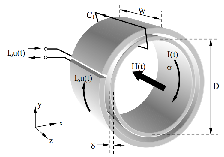
If the inner cylinder were a perfect conductor, then the current Iou(t) would produce an equal and opposite image current ~-Iou(t) on the outer surface of the inner cylinder, thus producing a net zero magnetic field inside the cylinder formed by that image current. Consider the integral of →H∙d→s around a closed contour C1 that threads both cylinders and circles zero net current at t = 0+; this integral yields zero. If the inner conductor were slightly resistive, then the same equal and opposite current would flow on the inner cylinder, but it would slowly dissipate heat until the image current decayed to zero and the magnetic field inside reached the maximum value Io/W [A m-1] associated with the outer current Io. These conclusions are quantified below.
The magnetic field H inside the inner cylinder depends on the currents flowing in the outer and inner cylinders, Io and I(t), respectively:
H(t)=u(t)[Io+I(t)]/W
The current I(t) flowing in the inner cylinder is driven by the voltage induced by H(t) via Faraday’s law (2.4.14):
∮C2→E∙d→s=IR=μo∫A(d→H/dt)∙d→a=μoAdH/dt
where the contour C2 is in the x-y plane and circles the inner cylinder with diameter D. The area circled by the contour A = πD2/4. The circumferential resistance of the inner cylinder is R = πD/σδW ohms. For simplicity we assume that the permeability here is μo everywhere. Substituting (4.3.11) into (4.3.12) yields a differential equation for I(t):
I(t)=−(μoA/WR)dI/dt
Substituting the general solution I(t) = Ke-t/τ into (4.3.13) yields:
Ke−t/τ=(μoA/WRτ)Ke−t/τ
τ=μ0A/WR=μ0Aσδ/πD[s](magnetic relaxation time)
Thus the greater the conductivity of the inner cylinder, and the larger its product μA, the longer it takes for transient magnetic fields to penetrate it. For the special case where δ = D/4π and A = D2 , we find τ = μoσ(D/2π)2 , which is the same magnetic relaxation time constant derived in (4.3.10) if we identify D with the wavelength λ of the magnetic field variations. Equation (4.3.15) is also approximately correct if μo → μ for the inner cylinder.
Since H(t) = 0 at t = 0+, (4.3.11) yields I(t = 0+) = - Io, and the solution I(t) = Ke-t/τ becomes:
I(t)=−Ioe−t/τ [A]
The magnetic field inside the inner cylinder follows from (4.3.16) and (4.3.11):
H(t)=u(t)Io(1−e−t/τ)/W[Am−1]
The geometry of Figure 4.3.1 can be used to heat resistive materials such as metals electrically by placing the metals in a ceramic container that sinusoidal magnetic fields penetrate easily. The induced currents can then melt the material quicker by heating the material throughout rather than just at the surface, as would a flame. The frequency f generally must be sufficiently low that the magnetic fields penetrate a significant fraction of the container diameter; f << 1/τ.
The inner cylinder of Figure 4.3.1 can also be used to shield its interior from alternating magnetic fields by designing it so that its time constant τ is much greater than the period of the undesired AC signal; large values of μσδ facilitate this since τ = μoAσδ/πD (4.3.15). Since we can model a solid inner cylinder as a continuum of concentric thin conducting shells, it follows that the inner shells will begin to see significant magnetic fields only after the surrounding shells do, and therefore the time delay experienced increases with depth. This is consistent with τ ∝ δ. The penetration of alternating fields into conducting surfaces is discussed further in Section 9.3 in terms of the exponential penetration skin depth δ=√2/ωμσ[m].
Two actuator configurations are suggested by Figure 4.3.1. First, the inner cylinder could be inserted only part way into the outer cylinder. Then the net force on the inner cylinder would expel it when the outer cylinder was energized because the polarity of these two electromagnets are reversed, the outer one powered by Io and the inner one by - Io(1 - e-t/τ ). Electromagnetic forces are discussed more fully in Chapter 5; here it suffices to note that induced currents can be used to simplify electromechanical actuators. A similar “kick” can be applied to a flat plate placed across the end of the outer cylinder, for again the induced cylindrically shaped mirror image current would experience a transient repulsive force. Mirror-image currents were discussed in Section 4.2.
The inner cores in transformers and some inductors are typically iron and are circled by wires carrying alternating currents, as discussed in Section 3.2. The alternating currents induce circular currents in the core called eddy currents that dissipate power. To minimize such induced currents and losses, high-μ conducting cores are commonly composed of many thin sheets separated from each other by thin coats of varnish or other insulator that largely blocks those induced currents; these are called laminated cores. A rough estimate of the effectiveness of using N plates instead of one can be obtained by noting that the power Pd dissipated in each lamination is proportional to V2/R, where V=∮C→E∙d→s is the loop voltage induced by H(t) and R is the effective resistance of that loop. By design H(t) usually penetrates the full transformer core. Thus V is roughly proportional to the area of each lamination in the plane perpendicular to →H, which decreases as 1/N. The resistance R experienced by the induced current circulating in each lamination increases roughly by N since the width of the channel through which it can flow is reduced as N increases while the length of the channel changes only moderately. The total power dissipated for N laminations is thus roughly proportional to NV2/R ∝ NN-2/N = N-2. Therefore we need only increase N to the point where the power loss is tolerable and the penetration of the transformer core by H(t) is nearly complete each period.
How long does it take a magnetic field to penetrate a 1-mm thick metal cylinder of diameter D with conductivity 5×10⁷ [S/m] if μ = μo? Design a shield for a ~10-cm computer that blocks 1 MHz magnetic fields emanating from an AM radio.
Solution
If we assume the geometry of Figure 4.3.1 and use (4.3.15), τ = μoAσδ/πD, we find τ = 1.3×10⁻⁶×D×5×107 ×10-3/4 = 0.016D seconds, where A = πD2/4 and δ = 10-3. If D = 0.1, then τ = 1.6×10⁻² seconds, which is ~105 longer than the rise time ~10-6/2π of a 1-MHz signal. If a smaller ratio of 102 is sufficient, then a one-micron thick layer of metal evaporated on thin plastic might suffice. If the metal had μ = 104 μo, then a onemicron thick layer would provide a safety factor of 106.