9.1: Waves at planar boundaries at normal incidence

Introduction to boundary value problems

Section 2.2 showed how uniform planes waves could propagate in any direction with any polarization, and could be superimposed in any combination to yield a total electromagnetic field. The general electromagnetic boundary value problem treated in Sections 9.1–4 involves determining exactly which, if any, combination of waves matches any given set of boundary conditions, which are the relations between the electric and magnetic fields adjacent to both sides of each boundary. These boundaries can generally be both active and passive, the active boundaries usually being sources. Boundary conditions generally constrain \(\overline{\mathrm{E}}\) and/or \(\overline{\mathrm{H}}\) for all time on the boundary of the two- or three-dimensional region of interest.

The uniqueness theorem presented in Section 2.8 states that only one solution satisfies all Maxwell’s equations if the boundary conditions are sufficient. Therefore we may solve boundary value problems simply by hypothesizing the correct combination of waves and testing it against Maxwell’s equations. That is, we leave undetermined the numerical constants that characterize the chosen combination of waves, and then determine which values of those constraints satisfy Maxwell’s equations. This strategy eases the challenge of hypothesizing the final answer directly. Moreover, symmetry and other considerations often suggest the nature of the wave combination required by the problem, thus reducing the numbers of unknown constants that must be determined.

The four basic steps for solving boundary value problems are:

1. Determine the natural behavior of each homogeneous section of the system in isolation (absent its boundaries).
2. Express this natural behavior as the superposition of waves characterized by unknown constants; symmetry and other considerations can minimize the number of waves required. Here our basic building blocks are usually uniform plane waves, but other more compact expansions are typically used if the symmetry of the problem permits, as illustrated in Section 4.5.2 for cylindrical and spherical geometries, Section 7.2.2 for TEM transmission lines, and Section 9.3.1 for waveguide modes.
3. Write equations for the boundary conditions that must be satisfied by these sets of superimposed waves, and then solve for the unknown constants.
4. Test the resulting solution against any of Maxwell’s equations that have not already been imposed.

Variations of this four-step procedure can be used to solve almost any problem by replacing Maxwell’s equations with their approximate equivalent for the given problem domain.

Reflection from perfect conductors

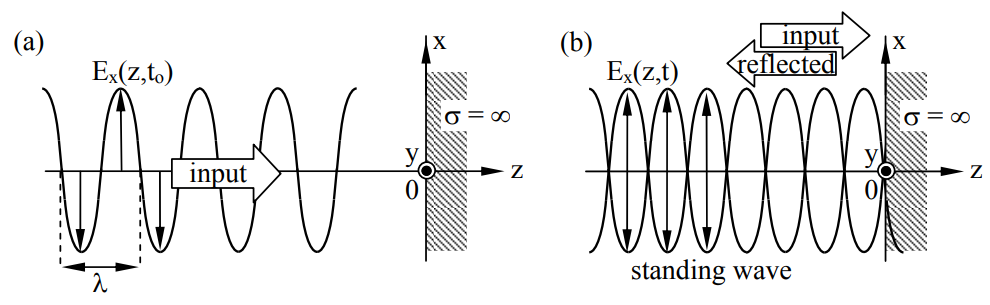
One of the simplest examples of a boundary value problem is that of a uniform plane wave in vacuum normally incident upon a planar perfect conductor at z ≥ 0, as illustrated in Figure 9.1.1(a). Step 1 of the general boundary-problem solution method of Section 9.1.2 is simply to note that electromagnetic fields in the medium can be represented by superimposed uniform plane waves.

Figure \(\PageIndex{1}\): Plane wave at normal incidence reflecting from a perfect conductor.

For this incompletely defined example, the initial part of Step 2 of the method involves refinement of the problem definition by describing more explicitly the incident wave, for example:

\[\overline{\mathrm{E}}(\mathrm{z}, \mathrm{t})=\hat{x} \mathrm{E}_{\mathrm{o}} \cos (\omega \mathrm{t}-\mathrm{kz}) \ \left[\mathrm{Vm}^{-1}\right]\]

where the wave number k = 2\(\pi\)/λ = ω/c = ω(μ_oε_o)^0.5, (2.3.24). The associated magnetic field (2.3.25) is:

\[\overline{\mathrm{H}}(\mathrm{z}, \mathrm{t})=\hat{y}\left(\mathrm{E}_{\mathrm{o}} / \eta_{\mathrm{o}}\right) \cos (\omega \mathrm{t}-\mathrm{kz}) \ \left[\mathrm{Am}^{-1}\right]\]

This unambiguously defines the source, and the boundary is similarly unambigous: σ = ∞ and therefore \(\overline{\mathrm{E}}=0\) for z ≥ 0. This more complete problem definition is sufficient to yield a unique solution. Often the first step in solving a problem is to ensure its definition is complete.

Since there can be no waves inside the perfect conductor, and since the source field alone does not satisfy the boundary condition \(\overline{\mathrm{E}}_{/ /}=0\) at z = 0, one or more additional plane waves must be superimposed to yield a valid solution. In particular, we need to match the boundary condition \(\overline{\mathrm{E}}_{/ /}=0\)at z = 0. This can be done by adding a single uniform plane wave propagating in the -z direction with an electric field that cancels the incident electric field at z = 0 for all time t. Thus we hypothesize that the total electric field is:

\[\overline{\mathrm{E}}(\mathrm{z}, \mathrm{t})=\hat{x}\left[\mathrm{E}_{\mathrm{o}} \cos (\omega \mathrm{t}-\mathrm{kz})+\mathrm{E}_{1} \cos (\omega \mathrm{t}+\mathrm{kz}+\phi)\right]\]

where we have introduced the constants E₁ and φ.

In Step 3 of the method we must solve the equation (9.1.3) that characterizes the boundary value constraints:

\[\overline{\mathrm{E}}(0, \mathrm{t})=\hat{x}\left[\mathrm{E}_{\mathrm{o}} \cos (\omega \mathrm{t}-0)+\mathrm{E}_{1} \cos (\omega\mathrm{t}+0+\phi)\right]=0\]

\[\therefore \mathrm{E}_{1}=-\mathrm{E}_{\mathrm{o}}, \phi=0\]

The result (9.1.5) yields the final trial solution:

\[\overline{\mathrm{E}}(\mathrm{z}, \mathrm{t})=\hat{x} \mathrm{E}_{\mathrm{o}}[\cos (\omega \mathrm{t}-\mathrm{kz})-\cos (\omega \mathrm{t}+\mathrm{kz})]=\hat{x} 2 \mathrm{E}_{\mathrm{o}}(\sin \omega \mathrm{t}) \sin \mathrm{kz}\]

\[\overline{\mathrm{H}}(z, t)=\hat{y} \mathrm{E}_{0}[\cos (\omega t-\mathrm{kz})+\cos (\omega t+\mathrm{kz})] / \eta_{\mathrm{o}}=\hat{y}\left(2 \mathrm{E}_{\mathrm{o}} / \eta_{\mathrm{o}}\right)(\cos \omega \mathrm{t}) \cos \mathrm{kz}\]

Note that the sign of the reflected \(\overline{\mathrm{H}}\) and wave is reversed from that of the reflected \(\overline{\mathrm{E}}\), consistent with the reversal of the Poynting vector for the reflected wave alone. We have used the identities:

\[\cos \alpha+\cos \beta=2 \cos [(\alpha+\beta) / 2] \cos [(\alpha-\beta) / 2]\]

\[\cos \alpha-\cos \beta=-2 \sin [(\alpha+\beta) / 2] \sin [(\alpha-\beta) / 2]\]

Also note that \(\overline{\mathrm{H}}(\mathrm{z}, \mathrm{t})\) is 90^o out of phase with \(\overline{\mathrm{E}}(\mathrm{z}, \mathrm{t}) \) with respect to both time and space.

We also need a trial solution for z > 0. Inside the conductor \(\overline{\mathrm{E}}=\overline{\mathrm{H}}=0\), and boundary conditions (2.6.17) require a surface current:

\[\overline{\mathrm{J}}_{\mathrm{S}}=\hat{n} \times \overline{\mathrm{H}} \ \left[\mathrm{Am}^{-1}\right]\]

The fourth and final step of this problem-solving method is to test the full trial solution against all of Maxwell’s equations. We know that our trial solution satisfies the wave equation in our source-free region because our solution is the superposition of waves that do; it therefore also satisfies Faraday’s and Ampere’s laws in a source-free region, as well as Gauss’s laws. At the perfectly conducting boundary we require \( \overline{\mathrm{E}}_{ / /}=0\) and \(\overline{\mathrm{H}}_{\perp}=0\); these constraints are also satisfied by our trial solution, and therefore the problem is solved for the vacuum. Zero-value fields inside the conductor satisfy all Maxwell’s equations, and the surface current \( \overline{\mathrm{J}}_{\mathrm{S}}\) (9.1.10) satisfies the final boundary condition.

The nature of this solution is interesting. Note that the total electric field is zero not only at the surface of the conductor, but also at a series of null planes parallel to the conductor and spaced at intervals Δ along the z axis such that kz_nulls = -n\(\pi\), where n = 0, 1, 2, ... That is, the null spacing Δ = \(\pi\)/k = λ/2, where λ is the wavelength. On the other hand, the magnetic field is maximum at those planes where E is zero (the null planes of E), and has nulls where E is maximum. Since the time average power flow and the Poynting vector are clearly zero at each of these planes, there is no net power flow to the right. Except at the field nulls, however, there is reactive power, as discussed in Section 2.7.3. Because no average power is flowing via these waves and the energy and waves are approximately stationary in space, the solution is called a standing wave, as illustrated in Figures 7.2.3 for VSWR and 7.4.1 for resonance on perfectly reflecting TEM transmission lines.

Reflection from transmissive boundaries

Often more than one wave must be added to the given incident wave to satisfy all boundary conditions. For example, assume the same uniform plane wave (9.1.1–2) in vacuum is incident upon the same planar interface, where a medium having μ,ε ≠ μ_o,ε_o for z ≥ 0 has replaced the conductor. We have no reason to suspect that the fields beyond the interface are zero, so we might try a trial solution with both a reflected wave E_r(z,t) and a transmitted wave E_t(z,t) having unknown amplitudes (E_r and E_t) and phases (φ and θ) for which we can solve:

\[\begin{align}&\overline{\mathrm{E}}(\mathrm{z}, \mathrm{t})=\hat{x}\left[\mathrm{E}_{\mathrm{o}} \cos (\omega \mathrm{t}-\mathrm{kz})+\mathrm{E}_{\mathrm{r}} \cos (\omega \mathrm{t}+\mathrm{kz}+\phi)\right] &\quad(\mathrm{z}<0)\\&\overline{\mathrm{E}}_{\mathrm{t}}(\mathrm{z}, \mathrm{t})=\hat{x} \mathrm{E}_{\mathrm{t}} \cos \left(\omega \mathrm{t}-\mathrm{k}_{\mathrm{t}} \mathrm{z}+\theta\right) & \text{(z ≥ 0)}\\&\overline{\mathrm{H}}(\mathrm{z}, \mathrm{t})=\hat{y}\left[\mathrm{E}_{\mathrm{o}} \cos (\omega \mathrm{t}-\mathrm{kz})-\mathrm{E}_{\mathrm{r}} \cos (\omega \mathrm{t}+\mathrm{kz}+\phi)\right] / \mathrm{\eta}_{\mathrm{o}} & \quad(\mathrm{z}<0)\\&\overline{\mathrm{H}}(\mathrm{z}, \mathrm{t})=\hat{y} \mathrm{E}_{\mathrm{t}} \cos \left(\omega \mathrm{t}-\mathrm{k}_{\mathrm{t}} \mathrm{z}+\theta\right) / \mathrm{\eta}_{\mathrm{t}} & \text{(z ≥ 0)}\end{align}\]

where \( \mathrm{k}=\omega \sqrt{\mu_{\mathrm{o}} \varepsilon_{\mathrm{o}}}\), \(\mathrm{k}_{\mathrm{t}}=\omega \sqrt{\mu \varepsilon} \), \(\eta_{\mathrm{o}}=\sqrt{\mu_{\mathrm{o}} / \varepsilon_{\mathrm{o}}} \), and \(\eta_{\mathrm{t}}=\sqrt{\mu / \varepsilon} \).

Using these four equations to match boundary conditions at z = 0 for \( \overline{\mathrm{E}}_{/ /}\) and \(\overline{\mathrm{H}}_{ / /} \), both of which are continuous across an insulating boundary, and dividing by E_o, yields:

\[\begin{align}&\hat{x}\left[\cos (\omega \mathrm{t})+\left(\mathrm{E}_{\mathrm{r}} / \mathrm{E}_{\mathrm{o}}\right) \cos (\omega \mathrm{t}+\phi)\right]=\hat{x}\left(\mathrm{E}_{\mathrm{t}} / \mathrm{E}_{\mathrm{o}}\right) \cos (\omega \mathrm{t}+\theta) \\&\hat{y}\left[\cos (\omega \mathrm{t})-\left(\mathrm{E}_{\mathrm{r}} / \mathrm{E}_{\mathrm{o}}\right) \cos (\omega \mathrm{t}+\phi)\right] / \eta_{\mathrm{o}}=\hat{y}\left[\left(\mathrm{E}_{\mathrm{t}} / \mathrm{E}_{\mathrm{o}}\right) \cos (\omega \mathrm{t}+\theta)\right] / \eta_{\mathrm{t}}\end{align}\]

First we note that for these equations to be satisfied for all time t we must have φ = θ = 0, unless we reverse the signs of E_r or E_t and let φ or θ = \(\pi\), respectively, which is equivalent.

Dividing these two equations by cos ωt yields:

\[1+\left(\mathrm{E}_{\mathrm{r}} / \mathrm{E}_{\mathrm{o}}\right)=\mathrm{E}_{\mathrm{t}} / \mathrm{E}_{\mathrm{o}}\]

\[\left[1-\left(\mathrm{E}_{\mathrm{r}} / \mathrm{E}_{\mathrm{o}}\right)\right] / \eta_{\mathrm{o}}=\left(\mathrm{E}_{\mathrm{t}} / \mathrm{E}_{\mathrm{o}}\right) / \eta_{\mathrm{t}}\]

These last two equations can easily be solved to yield the wave reflection coefficient and the wave transmission coefficient:

\[\mathrm{\frac{E_{r}}{E_{o}}=\frac{\left(\eta_{t} / \eta_{0}\right)-1}{\left(\eta_{t} / \eta_{0}\right)+1}} \qquad \qquad \qquad \text{(reflection coefficient) }\]

\[\mathrm{\frac{E_{t}}{E_{o}}=\frac{2 \eta_{t}}{\eta_{t}+\eta_{o}}} \qquad \qquad \qquad \text{(transmission coefficient)}\]

The wave transmission coefficient E_t/E_o follows from (9.1.17) and (9.1.19). When the characteristic impedance \(\eta_{\mathrm{t}}\) of the dielectric equals that of the incident medium, \(\eta_{\mathrm{o}}\), there are no reflections and the transmitted wave equals the incident wave. We then have an impedance match. These values for E_r/E_o and E_t/E_o can be substituted into (9.1.11–14) to yield the final solution for \( \overline{\mathrm{E}}(\mathrm{z}, \mathrm{t})\) and \( \overline{\mathrm{H}}(\mathrm{z}, \mathrm{t})\).

The last step of the four-step method for solving boundary value problems involves checking this solution against all Maxwell’s equations—they are satisfied.

Example \(\PageIndex{A}\)

A 1-Wm^-2 uniform plane wave in vacuum, \(\hat{x} \mathrm{E}_{+} \cos (\omega \mathrm{t}-\mathrm{kz})), is normally incident upon a planar dielectric with ε = 4ε_o. What fraction of the incident power P₊ is reflected? What is \(\overline{\mathrm{H}}(\mathrm{t})\) at the dielectric surface (z = 0)?

Solution

\(\mathrm{P}_{-} / \mathrm{P}_{+}=\left|\mathrm{E}_{-} / \mathrm{E}_{+}\right|^{2}=\left|\left(\eta_{\mathrm{t}}-\eta_{\mathrm{o}}\right) /\left(\eta_{\mathrm{t}}+\eta_{\mathrm{o}}\right)\right|^{2}\), using (5.1.19). Since \(\eta_{\mathrm{t}}=\sqrt{\mu_{\mathrm{o}} / 4 \varepsilon_{\mathrm{o}}}=\eta_{\mathrm{o}} / 2\), therefore: \(\left.\mathrm{P}_{-} / \mathrm{P}_{+}=\|\left(\eta_{\mathrm{o}} / 2\right)-\eta_{\mathrm{o}}\right] /\left[\left(\eta_{\mathrm{o}} / 2\right)+\eta_{\mathrm{o}}\right]^{2}=(-1 / 3)^{2}=1 / 9\). For the forward wave: \(\overline{\mathrm{E}}=\hat{x} \mathrm{E}_{+} \cos (\omega \mathrm{t}-\mathrm{kz})\) and \(\overline{\mathrm{H}}=\hat{y}\left(\mathrm{E}_{+} / \eta_{\mathrm{o}}\right) \cos (\omega \mathrm{t}-\mathrm{kz})\), where \(\left|\mathrm{E}_{+}\right|^{2} / 2 \eta_{\mathrm{o}}=1\), so \(\mathrm{E}_{+}=\left(2 \eta_{\mathrm{o}}\right)^{0.5}=(2 \times 377)^{0.5} \cong 27 \ [\mathrm{V} / \mathrm{m}]\) The sum of the incident and reflected magnetic fields at z = 0 is

\[\overline{\mathrm{H}}=\hat{y}\left(\mathrm{E}_{+} / \eta_{\mathrm{o}}\right)[\cos (\omega \mathrm{t})-(1 / 3) \cos (\omega \mathrm{t})]\cong \hat{y}(27 / 377)(2 / 3) \cos (\omega \mathrm{t})=0.48 \hat{y} \cos (\omega \mathrm{t}) \ \left[\mathrm{A} \mathrm{m}^{-1}\right] \nonumber\]