
12.3: Lasers
- Page ID
- 25039
\( \newcommand{\vecs}[1]{\overset { \scriptstyle \rightharpoonup} {\mathbf{#1}} } \)
\( \newcommand{\vecd}[1]{\overset{-\!-\!\rightharpoonup}{\vphantom{a}\smash {#1}}} \)
\( \newcommand{\dsum}{\displaystyle\sum\limits} \)
\( \newcommand{\dint}{\displaystyle\int\limits} \)
\( \newcommand{\dlim}{\displaystyle\lim\limits} \)
\( \newcommand{\id}{\mathrm{id}}\) \( \newcommand{\Span}{\mathrm{span}}\)
( \newcommand{\kernel}{\mathrm{null}\,}\) \( \newcommand{\range}{\mathrm{range}\,}\)
\( \newcommand{\RealPart}{\mathrm{Re}}\) \( \newcommand{\ImaginaryPart}{\mathrm{Im}}\)
\( \newcommand{\Argument}{\mathrm{Arg}}\) \( \newcommand{\norm}[1]{\| #1 \|}\)
\( \newcommand{\inner}[2]{\langle #1, #2 \rangle}\)
\( \newcommand{\Span}{\mathrm{span}}\)
\( \newcommand{\id}{\mathrm{id}}\)
\( \newcommand{\Span}{\mathrm{span}}\)
\( \newcommand{\kernel}{\mathrm{null}\,}\)
\( \newcommand{\range}{\mathrm{range}\,}\)
\( \newcommand{\RealPart}{\mathrm{Re}}\)
\( \newcommand{\ImaginaryPart}{\mathrm{Im}}\)
\( \newcommand{\Argument}{\mathrm{Arg}}\)
\( \newcommand{\norm}[1]{\| #1 \|}\)
\( \newcommand{\inner}[2]{\langle #1, #2 \rangle}\)
\( \newcommand{\Span}{\mathrm{span}}\) \( \newcommand{\AA}{\unicode[.8,0]{x212B}}\)
\( \newcommand{\vectorA}[1]{\vec{#1}} % arrow\)
\( \newcommand{\vectorAt}[1]{\vec{\text{#1}}} % arrow\)
\( \newcommand{\vectorB}[1]{\overset { \scriptstyle \rightharpoonup} {\mathbf{#1}} } \)
\( \newcommand{\vectorC}[1]{\textbf{#1}} \)
\( \newcommand{\vectorD}[1]{\overrightarrow{#1}} \)
\( \newcommand{\vectorDt}[1]{\overrightarrow{\text{#1}}} \)
\( \newcommand{\vectE}[1]{\overset{-\!-\!\rightharpoonup}{\vphantom{a}\smash{\mathbf {#1}}}} \)
\( \newcommand{\vecs}[1]{\overset { \scriptstyle \rightharpoonup} {\mathbf{#1}} } \)
\(\newcommand{\longvect}{\overrightarrow}\)
\( \newcommand{\vecd}[1]{\overset{-\!-\!\rightharpoonup}{\vphantom{a}\smash {#1}}} \)
\(\newcommand{\avec}{\mathbf a}\) \(\newcommand{\bvec}{\mathbf b}\) \(\newcommand{\cvec}{\mathbf c}\) \(\newcommand{\dvec}{\mathbf d}\) \(\newcommand{\dtil}{\widetilde{\mathbf d}}\) \(\newcommand{\evec}{\mathbf e}\) \(\newcommand{\fvec}{\mathbf f}\) \(\newcommand{\nvec}{\mathbf n}\) \(\newcommand{\pvec}{\mathbf p}\) \(\newcommand{\qvec}{\mathbf q}\) \(\newcommand{\svec}{\mathbf s}\) \(\newcommand{\tvec}{\mathbf t}\) \(\newcommand{\uvec}{\mathbf u}\) \(\newcommand{\vvec}{\mathbf v}\) \(\newcommand{\wvec}{\mathbf w}\) \(\newcommand{\xvec}{\mathbf x}\) \(\newcommand{\yvec}{\mathbf y}\) \(\newcommand{\zvec}{\mathbf z}\) \(\newcommand{\rvec}{\mathbf r}\) \(\newcommand{\mvec}{\mathbf m}\) \(\newcommand{\zerovec}{\mathbf 0}\) \(\newcommand{\onevec}{\mathbf 1}\) \(\newcommand{\real}{\mathbb R}\) \(\newcommand{\twovec}[2]{\left[\begin{array}{r}#1 \\ #2 \end{array}\right]}\) \(\newcommand{\ctwovec}[2]{\left[\begin{array}{c}#1 \\ #2 \end{array}\right]}\) \(\newcommand{\threevec}[3]{\left[\begin{array}{r}#1 \\ #2 \\ #3 \end{array}\right]}\) \(\newcommand{\cthreevec}[3]{\left[\begin{array}{c}#1 \\ #2 \\ #3 \end{array}\right]}\) \(\newcommand{\fourvec}[4]{\left[\begin{array}{r}#1 \\ #2 \\ #3 \\ #4 \end{array}\right]}\) \(\newcommand{\cfourvec}[4]{\left[\begin{array}{c}#1 \\ #2 \\ #3 \\ #4 \end{array}\right]}\) \(\newcommand{\fivevec}[5]{\left[\begin{array}{r}#1 \\ #2 \\ #3 \\ #4 \\ #5 \\ \end{array}\right]}\) \(\newcommand{\cfivevec}[5]{\left[\begin{array}{c}#1 \\ #2 \\ #3 \\ #4 \\ #5 \\ \end{array}\right]}\) \(\newcommand{\mattwo}[4]{\left[\begin{array}{rr}#1 \amp #2 \\ #3 \amp #4 \\ \end{array}\right]}\) \(\newcommand{\laspan}[1]{\text{Span}\{#1\}}\) \(\newcommand{\bcal}{\cal B}\) \(\newcommand{\ccal}{\cal C}\) \(\newcommand{\scal}{\cal S}\) \(\newcommand{\wcal}{\cal W}\) \(\newcommand{\ecal}{\cal E}\) \(\newcommand{\coords}[2]{\left\{#1\right\}_{#2}}\) \(\newcommand{\gray}[1]{\color{gray}{#1}}\) \(\newcommand{\lgray}[1]{\color{lightgray}{#1}}\) \(\newcommand{\rank}{\operatorname{rank}}\) \(\newcommand{\row}{\text{Row}}\) \(\newcommand{\col}{\text{Col}}\) \(\renewcommand{\row}{\text{Row}}\) \(\newcommand{\nul}{\text{Nul}}\) \(\newcommand{\var}{\text{Var}}\) \(\newcommand{\corr}{\text{corr}}\) \(\newcommand{\len}[1]{\left|#1\right|}\) \(\newcommand{\bbar}{\overline{\bvec}}\) \(\newcommand{\bhat}{\widehat{\bvec}}\) \(\newcommand{\bperp}{\bvec^\perp}\) \(\newcommand{\xhat}{\widehat{\xvec}}\) \(\newcommand{\vhat}{\widehat{\vvec}}\) \(\newcommand{\uhat}{\widehat{\uvec}}\) \(\newcommand{\what}{\widehat{\wvec}}\) \(\newcommand{\Sighat}{\widehat{\Sigma}}\) \(\newcommand{\lt}{<}\) \(\newcommand{\gt}{>}\) \(\newcommand{\amp}{&}\) \(\definecolor{fillinmathshade}{gray}{0.9}\)Physical principles of stimulated emission and laser amplification
Lasers (Light Amplification by Stimulated Emission of Radiation) amplify electromagnetic waves at wavelengths ranging from radio to ultraviolet and x-rays. They were originally called masers because the first units amplified only microwaves. Lasers can also oscillate when the amplified waves are reflected back into the device. The physical principles are similar at all wavelengths, though the details differ. Laser processes can occur in solids, liquids, or gases.
Lasers have a wide and growing array of applications. For example, optical fiber communications systems today commonly use Erbium-doped fiber amplifiers (EDFA’s) that amplify ~1.5-micron wavelength signals having bandwidths up to ~4 THz. Semiconductor, gas, and glass fiber laser amplifiers are also used to communicate within single pieces of equipment and for local fiber or free-space communications. Lasers also generate coherent beams of light used for measuring distances and angles; recording and reading data from memory devices such as CD’s and DVD’s; and for cutting, welding, and shaping materials, including even the human eye. Laser pointers have been added to pocket pens while higher-power industrial units can cut steel plates several inches thick. Weapons and laser-driven nuclear fusion reactions require still higher-power lasers. Peak laser pulse powers can exceed 1015 watts, a thousand times the total U.S. electrical generating capacity of ~5×10¹¹ watts. The electric field strengths within a focal spot of <100-micron diameter can strip electrons from atoms and accelerate them to highly relativistic velocities within a single cycle of the radiation. The roles of lasers in science, medicine, industry, consumer products, and other fields are still being defined.
Laser operation depends intimately upon the quantum nature of matter and the fact that charges trapped in atoms and molecules generally move at constant energy without radiating. Instead, transitions between atomic or molecular energy states occur abruptly, releasing or absorbing a photon.69 This process and lasers can fortunately be understood semi-classically without reference to a full quantum description.
Electrons within atoms, molecules, and crystals occupy discrete energy states; the lower energy states are preferentially occupied. Energy states can also be vibrational, rotational, magnetic, chemical, nuclear, etc.70 The number of possible states greatly exceeds those that are occupied.
69 Alternatively, acoustic phonons with energy hf can be released or absorbed, or an additional molecular or atomic state transition can occur to conserve energy. Phonons are acoustic quanta associated with mechanical waves in materials. Optical transitions can also absorb or emit two photons with total energy equal to Ε2 − Ε1, although such two-photon transitions are much less likely.
70 The distances between adjacent nuclei in molecules can oscillate sinusoidally with quantized amplitudes and frequencies characterisitic of each vibrational state. Isolated molecules can spin at specific frequencies corresponding to various rotational energy states. Electron spins and orbits together have magnetic dipole moments that align with or oppose an applied magnetic field to a quantized degree. Atoms bond to one another in quantized ways having specific chemical consequences. Nuclear magnetic moments can also align with other atomic or molecular magnetic moments in quantized ways corresponding to discrete energy states.
For example, as illustrated in Figure 12.3.1(a), an electron trapped in an atom, molecule, or crystal with energy E1 can be excited into any vacant higher-energy state (E2) by absorbing a photon of frequency f and energy ΔE where:
\[\Delta \mathrm{E}=\mathrm{E}_{2}-\mathrm{E}_{1}=\mathrm{hf} \ [\mathrm{J}] \label{12.3.1} \]
The constant h is Planck’s constant (6.625×10⁻³⁴ [Js]), and the small circles in the figure represent electrons in specific energy states.
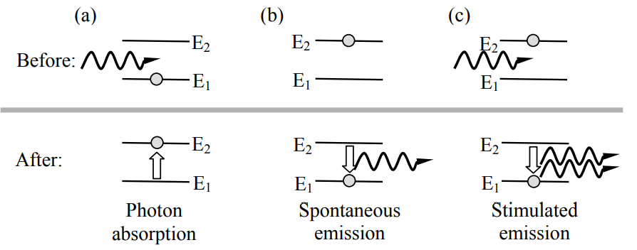
Figures 12.3.1(b) and (c) illustrate two additional basic photon processes: spontaneous emission and stimulated emission. Photon absorption (a) occurs with a probability that depends on the photon flux density [Wm-2], frequency [Hz], and the cross-section for the energy transition of interest. Spontaneous emission of photons (b) occurs with a probability A that depends only on the transition, as discussed below. Stimulated emission (c) occurs when an incoming photon triggers emission of a second photon; the emitted photon is always exactly in phase with the first, and propagates in the same direction. Laser action depends entirely on this third process of stimulated emission, while the first two processes often weaken it.
The net effect of all three processes—absorption, spontaneous emission, and stimulated emission—is to alter the relative populations, N1 and N2, of the two energy levels of interest. An example exhibiting these processes is the Erbium-doped fiber amplifiers commonly used to amplify optical telecommunications signals near 1.4-micron wavelength on long lines. Figure 12.3.2 illustrates how an optical fiber with numerous atoms excited by an optical pump (discussed further below) can amplify input signals at the proper frequency. Since the number of excited atoms stimulated to emit is proportional to the input wave intensity, perhaps only one atom might be stimulated to emit initially (because the input signal is weak), producing two inphase photons—the original plus the one stimulated. These two then propagate further stimulating two emissions so as to yield four in-phase photons.
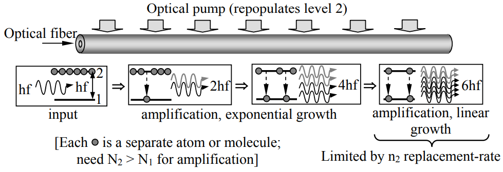
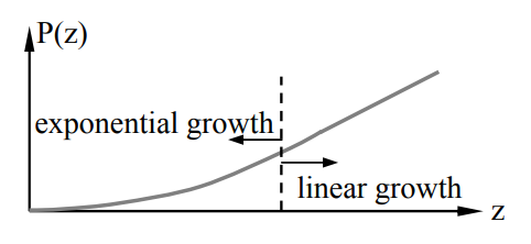
This exponential growth continues until the pump can no longer empty E1 and refill E2 fast enough; as a result absorption [m-1] approaches emission [m-1] as N1 approaches N2 locally. In this limit the increase in the number of photons per unit length is limited by the number np of electrons pumped from E1 to E2 per unit length. Thereafter the signal strength then increases only linearly with distance rather than exponentially, as suggested in Figure 12.3.3; the power increase per unit length then approaches nphf [Wm-1].
Simple equations characterize this process quantitatively. If E1 < E2 were the only two levels in the system, then:
\[\mathrm{d} \mathrm{N}_{2} / \mathrm{dt}=-\mathrm{A}_{21} \mathrm{N}_{2}-\mathrm{I}_{21} \mathrm{B}_{21}\left(\mathrm{N}_{2}-\mathrm{N}_{1}\right)\ \left[\mathrm{s}^{-1}\right] \label{12.3.2} \]
The probability of spontaneous emission from E2 to E1 is A21, where \(\tau_{21}=1 / \mathrm{A}_{21}\) is the 1/e lifetime of state E2. The intensity of the incident radiation at f = (E2-E1)/h [Hz] is:
\[\mathrm{I}_{21}=\mathrm{F}_{21} \mathrm{hf} \ \left[\mathrm{Wm}^{-2}\right] \label{12.3.3} \]
where F21 is the photon flux [photons m-2s-1] at frequency f. The right-most term of (12.3.2) corresponds to the difference between the number of stimulated emissions (∝ N2) and absorptions (∝ N1), where the rate coefficients are:
\[\mathrm{B}_{21}=\mathrm{A}_{21}\left(\pi^{2} \mathrm{c}^{2} / \mathrm{h} \omega^{3} \mathrm{n}^{2}\right)\left[\mathrm{m}^{2} \ \mathrm{J}^{-1}\right] \label{12.3.4} \]
\[\mathrm{A}_{21}=2 \omega^{3} \mathrm{D}_{21}^{2} / \mathrm{hsc}^{3} \ \left[\mathrm{s}^{-1}\right] \label{12.3.5} \]
In these equations n is the index of refraction of the fiber and D21 is the quantum mechanical electric or magnetic dipole moment specific to the state-pair 2,1. It is the sharply varying values of the dipole moment Dij from one pair of levels to another that makes pumping practical, as explained below.
Laser amplification can occur only when N2 exceeds N1, but in a two-level system no pump excitation can accomplish this; even infinitely strong incident radiation I21 at the proper frequency can only equalize the two populations via (\ref{12.3.2}).71 Instead, three- or four-level lasers are generally used. The general principle is illustrated by the three-level laser of Figure 12.3.4(a), for which the optical laser pump radiation driving the 1,3 transition is so strong that it roughly equalizes N1 and N3. The key to this laser is that the spontaneous rate of emission A32 >> A21 so that all the active atoms quickly accumulate in the metastable long-lived level 2 in the absence of stimulation at f21. This generally requires D32 >> D21, and finding materials with such properties for a desired laser frequency can be challenging.
71 Two-level lasers have been built, however, by physically separating the excited atoms or molecules from the unexcited ones. For example, excited ammonia molecules can be separated from unexcited ones by virtue of their difference in deflection when a beam of such atoms in vacuum passes through an electric field gradient.
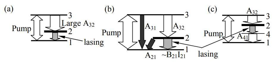
Since it requires hf13 Joules to raise each atom to level 3, and only hf21 Joules emerges as amplified additional radiation, the power efficiency \(\eta\) (power out/power in) cannot exceed the intrinsic limit \(\eta_{\mathrm{I}}=\mathrm{f}_{21} / \mathrm{f}_{31}\). In fact the efficiency is lowered further by a factor of \(\eta_{\mathrm{A}}\) corresponding to spontaneous emission from level 3 directly to level 1, bypassing level 2 as suggested in Figure 12.3.4(b), and to the spontaneous decay rate A21 which produces radiation that is not coherent with the incoming signal and radiates in all directions. Finally, only a fraction \(\eta_{\mathrm{p}}\) of the pump photons are absorbed by the transition 1→2. Thus the maximum power efficiency for this laser in the absence of propagation losses is:
\[\eta=\eta_{\mathrm{I}} \eta_{\mathrm{A}} \eta_{\mathrm{p}} \label{12.3.6} \]
Figure 12.3.4(c) suggests a typical design for a four-level laser, where both A32 and A41 are much greater than A24 or A21 so that energy level 2 is metastable and most atoms accumulate there in the absence of strong radiation at frequency f24 or f21. The strong pump radiation can come from a laser, flash lamp, or other strong radiation source. Sunlight, chemical reactions, nuclear radiation, and electrical currents in gases pump some systems.
The ω3 dependence of A21 (\ref{12.3.5}) has a profound effect on maser and laser action. For example, any two-level maser or laser must excite enough atoms to level 2 to equal the sum of the stimulated and spontaneous decay rates. Since the spontaneous decay rate increases with ω3, the pump power must also increase with ω3 times the energy hf of each excited photon. Thus pump power requirements increase very roughly with ω4, making construction of x-ray or gamma-ray lasers extremely difficult without exceptionally high pump powers; even ultraviolet lasers pose a challenge. Conversely, at radio wavelengths the spontaneous rates of decay are so extremely small that exceedingly low pump powers suffice, as they sometimes do in the vast darkness of interstellar space.
Many types of astrophysical masers exist in low-density interstellar gases containing H2O, OH, CO, and other molecules. They are typically pumped by radiation from nearby stars or by collisions occurring in shock waves. Sometimes these lasers radiate radially from stars, amplifying starlight, and sometimes they spontaneously radiate tangentially along linear circumstellar paths that have minimal relative Doppler shifts. Laser or maser action can also occur in darkness far from stars as a result of molecular collisions. The detailed frequency, spatial, and time structures observed in astrophysical masers offer unique insights into a wide range of astrophysical phenomena.
What is the ratio of laser output power to pump power for a three-level laser like that shown in Figure 12.3.4(a) if: 1) all pump power is absorbed by the 1→3 transition, 2) N2 >> N1, 3) A21/I21B21 = 0.1, 4) A31 = 0.1A32, and 5) f31 = 4f21?
Solution
The desired ratio is the efficiency \(\eta \) of (12.3.6) where the intrinsic efficiency is \( \eta_{\mathrm{I}}=\mathrm{f}_{21} / \mathrm{f}_{31}=0.25\), and the pump absorption efficiency \(\eta_{\mathrm{p}}=1\). The efficiency \( \eta_{\mathrm{A}}\) is less than unity because of two small energy losses: the ratio A31/A32 = 0.1, and the ratio A21/I21B21 = 0.1. Therefore \( \eta_{\mathrm{A}}=0.9^{2}=0.81\), and \( \eta=\eta_{1} \eta_{\mathrm{A}} \eta_{\mathrm{p}}=0.25 \times 0.81 \cong 0.20\).
Laser oscillators
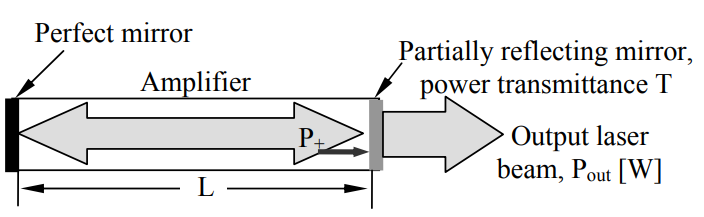
Laser amplifiers oscillate nearly monochromatically if an adequate fraction of the amplified signal is reflected back to be amplified further. For example, the laser oscillator pictured in Figure 12.3.5 has parallel mirrors at both ends of a laser amplifier, separated by L meters. One mirror is perfect and the other transmits a fraction T (say ~0.1) of the incident laser power. The roundtrip gain in the absence of loss is e2gL. This system oscillates if the net roundtrip gain at any frequency exceeds unity, where round-trip absorption (\(e^{-2 \alpha L}\)) and the partially transmitting mirror account for most loss.
Amplifiers at the threshold of oscillation are usually in their exponential region, so this net roundtrip gain exceeds unity when:
\[\mathrm{(1-T) e^{2(g-\alpha) L}>1} \label{12.3.7} \]
Equation (\ref{12.3.7}) implies \(\mathrm{e}^{2(\mathrm{g}-\alpha) \mathrm{L}} \geq(1-\mathrm{T})^{-1} \) for oscillation to occur. Generally the gain g per meter is designed to be as high as practical, and then L and T are chosen to be consistent with the desired output power. The pump power must be above the minimum threshold that yields g > \(\alpha\).
The output power from such an oscillator is simply Pout = TP+ watts, and depends on pump power Ppump and laser efficiency. Therefore:
\[\mathrm{P}_{+}=\mathrm{P}_{\text {out }} / \mathrm{T}=\eta \mathrm{P}_{\text {pump }} / \mathrm{T} \label{12.3.8} \]
Thus small values of T simply result in higher values of P+, which can be limited by internet breakdown or failure.
One approach to obtaining extremely high laser pulse powers is to abruptly increase the Q (reverberation) of the laser resonator after the pump source has fully populated the upper energy level. To prevent lasing before that level is fully populated, strong absorption can be introduced in the round-trip laser path to prevent amplification of any stimulated emission. The instant the absorption ceases, i.e. after Q-switching, the average round-trip gain g of the laser per meter exceeds the average absorption \(\alpha\) and oscillation commences. At high Q values lasing action is rapid and intense, so the entire upper population is encouraged to emit instantly, particularly if the lower level can be rapidly emptied. Such a device is called a Q-switched laser. Resonator Q is discussed further in Section 7.8.
The electronic states of glass fiber amplifiers are usually associated with quantized electron orbits around the added Erbium atoms, and state transitions simply involve electron transfers between two atomic orbits having different energies. In contrast, the most common lasers are laser diodes, which are transparent semiconductor p-n junctions for which the electron energy transitions occur between the conduction and valence bands, as suggested in Figure 12.3.6.
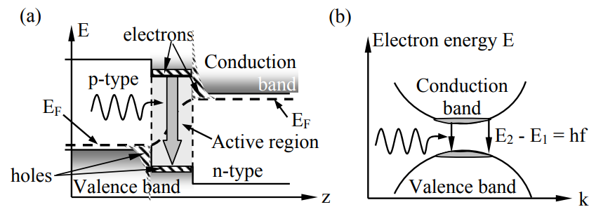
Parallel mirrors at the sides of the p-n junction partially trap the laser energy, forming an oscillator that radiates perpendicular to the mirrors; one of the mirrors is semi-transparent. Strong emission does not occur in any other direction because without the mirrors there is no feedback. Such lasers are pumped by forward-biasing the diode so that electrons thermally excited into the n-type conduction band diffuse into the active region where photons can stimulate emission, yielding amplification and oscillation within the ~0.2-μm thick p-n junction. Vacancies in the valence band are provided by the holes that diffuse into the active region from the p-type region. Voltage-modulated laser diodes can produce digital pulse streams at rates above 100 Mbps.
The vertical axis E of Figure 12.3.6(a) is electron energy and the horizontal axis is position z through the diode from the p to n sides of the junction. The exponentials suggest the Boltzmann energy distributions of the holes and electrons in the valence and conduction bands, respectively. Below the Fermi level, EF, energy states have a high probability of being occupied by electrons; EF(z) tilts up toward the right because of the voltage drop from the p-side to the n-side. Figure 12.3.6(b) plots electron energy E versus the magnitude of the k vector for electrons (quantum approaches treat electrons as waves characterized by their wavenumber k), and suggests why diode lasers can have broad bandwidths: the energy band curvature with k broadens the laser linewidth Δf. Incoming photons can stimulate any electron in the conduction band to decay to any empty level (hole) in the valence band, and both of these bands have significant energy spreads ΔE, where the linewidth Δf ≅ ΔE/h [Hz].
The resonant frequencies of laser diode oscillators are determined by E2 - E1, the linewidth of that transition, and by the resonant frequencies of the TEM mirror cavity resonator. The width Δω of each resonance is discussed further later. If the mirrors are perfect conductors that force \(\overrightarrow{\mathrm{E}}_{/ /}=0\), then there must be an integral number m of half wavelengths within the cavity length L so that \( \mathrm{m} \lambda_{\mathrm{m}}=2 \mathrm{L}\). The wavelength \( \lambda_{\mathrm{m}}^{\prime}\) is typically shorter than the free-space wavelength \( \lambda_{\mathrm{m}}\) due to the index of refraction n of the laser material. Therefore \(\lambda_{\mathrm{m}}=2 \mathrm{Ln} / \mathrm{m}=\mathrm{c} / \mathrm{f}_{\mathrm{m}} \), and:
\[\mathrm{f}_{\mathrm{m}}=\mathrm{cm} / 2 \mathrm{Ln} \label{12.3.9} \]
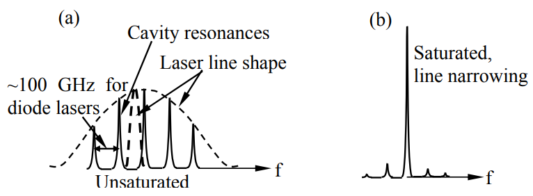
For typical laser diodes L and n might be 0.5 mm and 3, respectively, yielding a spacing between cavity resonances of: c/2Ln = 3×10⁸ /(2×10-3×1.5) = 100 GHz, as suggested in Figure 12.3.7(a). The figure suggests how the natural (atomic) laser line width might accommodate multiple cavity resonances, or possibly only one.
If the amplifier line shape is narrow compared to the spacing between cavity resonances, then the cavity length L might require adjustment in order to place one of the cavity resonances on the line center before oscillations occur. The line width of a laser depends on the widths of the associated energy levels Ei and Ej. These can be quite broad, as suggested by the laser diode energy bands illustrated in Figure 12.3.6(b), or quite narrow. Similarly, the atoms in an EDFA are each subject to slightly different local electrical fields due to the random nature of the glassy structure in which they are imbedded. This results in each atom having slightly different values for Ei so that EFDA’s amplify over bandwidths much larger than the bandwidth of any single atom.
Lasers for which each atom has its own slightly displaced resonant frequency due to local fields are said to exhibit inhomogeneous line broadening. In contrast, many lasers have no such frequency spread induced by local factors, so that all excited atoms exhibit the same line center and width; these are said to exhibit homogeneous line broadening. The significance of this difference is that when laser amplifiers are saturated and operate in their linear growth region, homogeneously broadened lasers permit the strongest cavity resonance within the natural line width to capture most of the energy available from the laser pump, suppressing the rest of the emission and narrowing the line, as suggested in Figure 12.3.7(b). This suppression of weak resonances is reduced in inhomogeneously broadened lasers because all atoms are pumped equally and have their own frequency sub-bands where they amplify independently within the natural line width.
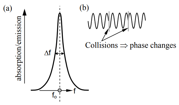
In gases the width of any spectral line is also controlled by the frequency of molecular collisions. Figure 12.3.8(b) illustrates how an atom or molecule with sinusoidal time variations in its dipole moment might be interrupted by collisions that randomly reset the phase. An electromagnetic wave interacting with this atom or molecule would then see a less pure sinusoid. This new spectral characteristic would no longer be a spectral impulse, i.e., the Fourier transform of a pure sinusoid, but rather the transform of a randomly interrupted sinusoid, which has the Lorentz line shape illustrated in Figure 12.3.8(a). Its half-power width is Δf, which is approximately the collision frequency divided by 2\(\pi\). The limited lifetime of an atom or molecule in any state due to the probability A of spontaneous emission results in similar broadening, where Δf ≅ A/2\(\pi\); this is called the intrinsic linewidth of that transition.
A Q-switched 1-micron wavelength laser of length L = 1 mm is doped with 1018 active atoms all pumped to their upper state. When the Q switches instantly to 100, approximately what is the maximum laser power output P [W]? Assume \(\varepsilon=4 \varepsilon_{0}\).
Solution
The total energy released when the Q switches is 1018hf ≅ 1018 × 6.6×10-34 × 3×1014 = 0.20 Joules. If the laser gain is sufficiently high, then a triggering photon originating near the output could be fully amplified by the time the beam reaches the rear of the laser, so that all atoms would be excited as that reflected pulse emerges from the front of the laser. A triggering photon at the rear of the laser would leave some atoms unexcited. Thus the minimum time for full energy release lies between one and two transit times \(\tau \) of the laser, depending on its gain; \( \tau=\mathrm{L} / \mathrm{c}^{\prime}=2 \mathrm{L} / \mathrm{c}=6.7 \times 10^{-12}\). Lower laser gains may require many transit times before all atoms are stimulated to emit. Therefore P < ~0.2/(6.7×10-12) ≅ 30 GW.