14.2: Complex Numbers and Sinusoidal Representation

Most linear systems that store energy exhibit frequency dependence and therefore are more easily characterized by their response to sinusoids rather than to arbitrary waveforms. The resulting system equations contain many instances of $A\cos(ωt + \phi$), where $A$, $ω$, and $\phi$ are the amplitude, frequency, and phase of the sinusoid, respectively. $A\cos(ωt + \phi$) can be replaced by $\underline{\mathrm{A}}$ using complex notation, indicated here by the underbar and reviewed below; it utilizes the arbitrary definition:

$$j \equiv(-1)^{0.5} \label{B.1} \tag{B.1}$$

This arbitrary non-physical definition is exploited by De Moivre’s theorem ($\ref{B.4}$), which utilizes a unique property of e = 2.71828:

$$\mathrm{e}^{\phi}=1+\phi+\phi^{2} / 2 !+\phi^{3} / 3 !+\ldots \tag{B.2}$$

Therefore:

$$\begin{align} \mathrm{e}^{\mathrm{j} \phi} &=1+\mathrm{j} \phi-\phi^{2} / 2 !-\mathrm{j} \phi^{3} / 3 !+\phi^{4} / 4 !+\mathrm{j} \phi^{5} / 5 !-\ldots \nonumber \\ &=\left[1-\phi^{2} / 2 !+\phi^{4} / 4 !-\ldots\right]+\left[\mathrm{j} \phi-\mathrm{j} \phi^{3} / 3 !+\mathrm{j} \phi^{5} / 5 ! \ldots\right] \tag{B.3} \end{align} \nonumber$$

$$\mathrm{e}^{\mathrm{j} \phi}=\cos \phi+\mathrm{j} \sin \phi \label{B.4} \tag{B.4}$$

This is a special instance of a general complex number $\underline{\mathrm{A}}$:

$$\underline{\mathrm{A}}=\mathrm{A}_{\mathrm{r}}+\mathrm{j} \mathrm{A}_{\mathrm{i}} \label{B.5} \tag{B.5}$$

where the real part is $\mathrm{A_{r} \equiv R_{e}\{\underline A\}}$ and the imaginary part is $\mathrm{A}_{\mathrm{i}} \equiv \mathrm{I}_{\mathrm{m}}\{\mathrm{\underline A}\}$.

It is now easy to use ($\ref{B.4}$) and ($\ref{B.5}$) to show that⁷⁶:

$$\operatorname{Acos}(\omega \mathrm{t}+\phi)=\mathrm{R}_{\mathrm{e}}\left\{\mathrm{Ae}^{\mathrm{j}(\omega \mathrm{t}+\phi)}\right\}=\mathrm{R}_{\mathrm{e}}\left\{\mathrm{Ae}^{\mathrm{j} \phi} \mathrm{e}^{\mathrm{j} \omega \mathrm{t}}\right\}=\mathrm{R}_{\mathrm{e}}\left\{\mathrm{Ae}^{\mathrm{j} \omega \mathrm{t}}\right\}=\mathrm{A}_{\mathrm{r}} \cos \omega \mathrm{t}-\mathrm{A}_{\mathrm{i}} \sin \omega \mathrm{t} \label{B.6} \tag{B.6}$$

where:

$$\underline{\mathrm{A}}=\mathrm{Ae}^{\mathrm{j} \phi}=\mathrm{A} \cos \phi+\mathrm{j} \mathrm{A} \sin \phi=\mathrm{A}_{\mathrm{r}}+\mathrm{j} \mathrm{A}_{\mathrm{i}} \label{B.7} \tag{B.7}$$

$$\mathrm{A_{r} \equiv \operatorname{Acos} \phi, \quad A_{i} \equiv A \sin \phi} \label{B.8} \tag{B.8}$$

⁷⁶ The physics community differs and commonly defines $\operatorname{Acos}(\omega \mathrm{t}+\phi)=\mathrm{R}_{\mathrm{e}}\left\{\mathrm{Ae}^{-\mathrm{j}(\omega \mathrm t+\phi)}\right\}$ and $\mathrm{A_{i} \equiv-A \sin \phi}$, where the rotational direction of $\phi$ is reversed in Figure 14.2.1. Because phase is reversed in this alternative notation, the impedance of an inductor L becomes -jωL, and that of a capacitor becomes j/ωC. In this notation j is commonly replaced by -i.

The definition of $\underline{\mathrm{A}}$ given in ($\ref{B.8}$) has the useful geometric interpretation shown in Figure 14.2.1(a), where the magnitude of the phasor $\underline{\mathrm{A}}$ is simply the given amplitude A of the sinusoid, and the angle $\phi$ is its phase.

Figure $\PageIndex{1}$: Representation of phasors in the complex plane.

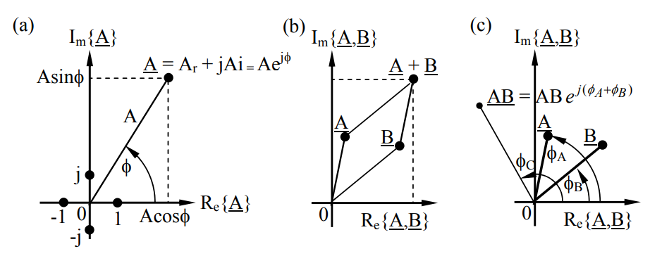
When $\phi$ = 0 we have $\mathrm{R}_{\mathrm{e}}\left\{\mathrm{\underline{A}e}^{\mathrm{j} \omega \mathrm{t}}\right\}=\mathrm{A} \cos \omega \mathrm{t}$, and when $\phi$ = $\pi$/2 we have -Asinωt. Advances in time alter the phasor $\underline{\mathrm{A}}$ in the same sense as advances in $\phi$; the phasor rotates counterclockwise. The utility of this diagram is partly that the signal of interest, $\mathrm{R}_{\mathrm{e}}\left\{\underline{\mathrm{A}} \mathrm{e}^{\mathrm{j} \omega \mathrm{t}}\right\}$, is simply the projection of the phasor $\mathrm{\underline{A}e}^{\mathrm{j} \omega \mathrm{t}}$ on the real axis. It also makes clear that:

$$\mathrm{A}=\left(\mathrm{A}_{\mathrm{r}}^{2}+\mathrm{A}_{\mathrm{i}}^{2}\right)^{0.5} \label{B.9} \tag{B.9}$$

$$\phi=\tan ^{-1}\left(\mathrm{A_{i} / A_{r}}\right) \tag{B.10} \label{B.10}$$

It is also easy to see, for example, that $\mathrm{e}^{\mathrm{j} \pi}=-1$, and that $\mathrm{\underline{A}=j A}$ corresponds to -Asinωt.

Examples of equivalent representations in the time and complex domains are:

$$\begin{aligned} \operatorname{Acos} \omega t & \leftrightarrow \mathrm{A} \\ -\mathrm{Asin} \omega \mathrm{t} & \leftrightarrow \mathrm{jA} \\ \mathrm{Acos}(\omega t+\phi) & \leftrightarrow \mathrm{Ae}^{\mathrm{j} \phi} \\ \mathrm{Asin}(\omega \mathrm{t}+\phi) & \leftrightarrow-\mathrm{jAe}^{\mathrm{j} \phi}=\mathrm{Ae}^{\mathrm{j}(\phi-\pi / 2)} \end{aligned} \nonumber$$

Complex numbers behave as vectors in some respects, where addition and multiplication are also illustrated in Figure 14.2.1(b) and (c), respectively:

$$\underline{\mathrm{A}}+\underline{\mathrm{B}}=\underline{\mathrm{B}}+\underline{\mathrm{A}}=\mathrm{A}_{\mathrm{r}}+\mathrm{B}_{\mathrm{r}}+\mathrm j\left(\mathrm{A}_{\mathrm{i}}+\mathrm{B}_{\mathrm{i}}\right) \label{B.11} \tag{B.11}$$

$$\underline{\mathrm{AB}}=\underline{\mathrm{BA}}=\left(\mathrm{A}_{\mathrm{r}} \mathrm{B}_{\mathrm{r}}-\mathrm{A}_{\mathrm{i}} \mathrm{B}_{\mathrm{i}}\right)+j\left(\mathrm{A}_{\mathrm{r}} \mathrm{B}_{\mathrm{i}}+\mathrm{A}_{\mathrm{i}} \mathrm{B}_{\mathrm{r}}\right)=\mathrm{ABe}^{\mathrm{j}\left(\phi_{\mathrm{A}}+\phi_{\mathrm{B}}\right)} \label{B.12} \tag{B.12}$$

$$\underline{\mathrm{A}}^{*}=\mathrm{A}_{\mathrm{r}}-\mathrm{j} \mathrm{A}_{\mathrm{i}}=\mathrm{A} \mathrm{e}^{-\mathrm{j} \phi_{\mathrm{A}}} \label{B.13} \tag{B.13}$$

We can easily solve for the real and imaginary parts of $\underline{\mathrm{A}}$:

$$\mathrm{A_{r}=\left(\underline{A}+\underline{A}^{*}\right) / 2, \quad A_{i}=\left(\underline{A}-\underline{A}^{*}\right) / 2} \label{B.14} \tag{B.14}$$

Ratios of complex numbers can also be readily computed:

$$\mathrm{\underline A} / \mathrm{\underline B}=(\mathrm{\underline A} / \mathrm{\underline B}) \mathrm{e}^{\mathrm{j}\left(\phi_{\mathrm{A}}-\phi_{\mathrm{B}}\right)}=\mathrm{\underline{A} \underline{B}}^{*} / \mathrm{\underline{BB}}^{*}=\mathrm{\underline{AB}}^{*} /|\mathrm{\underline{B}}|^{2} \tag{B.15} \label{B.15}$$

Even an n^th root of $\underline{\mathrm{A}}=\mathrm{Ae}^{\mathrm{j} \phi}$ can be simply found:

$$\underline{\mathrm{A}}^{1 / \mathrm{n}}=\mathrm{A}^{1 / \mathrm{n}} \mathrm{e}^{\mathrm{j} \phi / \mathrm{n}} \label{B.16} \tag{B.16}$$

where n legitimate roots exist and are:

$$\underline{\mathrm{A}}^{1 / \mathrm{n}}=\mathrm{A}^{(1 / \mathrm{n})} \mathrm{e}^{(\mathrm{j} \phi / \mathrm{n})} \mathrm{e}^{(\mathrm{j} 2 \pi \mathrm{m} / \mathrm{n})} \label{B.17} \tag{B.17}$$

for m = 0, 1, …, n – 1.