
10.4: Antenna Arrays


- Last updated
- Jun 7, 2025
- Save as PDF

( \newcommand{\kernel}{\mathrm{null}\,}\)
Two-dipole arrays
Although some communications services such as mobile phones use nearly omnidirectional electric or magnetic dipole antennas (short-dipole and loop antennas), most fixed services such as point-to-point, broadcast, and satellite services benefit from larger antenna gains. Also, some applications require rapid steering of the antenna beam from one point to another, or even the ability to observe or transmit in multiple narrow directions simultaneously. Antenna arrays with two or more dipoles can support all of these needs. Arrays of other types of antennas can similarly boost performance.
Since the effective area of an antenna, A(θ,ϕ), is simply related by (10.3.36) to antenna gain G(θ,ϕ), the gain of a dipole array fully characterizes its behavior, which is determined by the array current distribution. Sometimes some of the dipoles are simply mirrored images of others.
In every case the total radiated field is simply the superposition of the fields radiated by each contributing dipole in proportion to its strength, and delayed in proportion to its distance from the observer. For two-dipole arrays, the differential path length to the receiver can lead to reinforcement if the two sinusoidal waves are in phase, cancellation if they are 180o out of phase and equal, and intermediate strength otherwise.
It is convenient to represent the signals as phasors since the patterns are frequency dependent, so the total observed electric field →E_=∑i→E_i, where →E_i is the observed contribution from short-dipole i, including its associated phase lag of γi radians due to distance traveled. Consider first the two-dipole array in Figure 10.4.1(a), where the dipoles are z-axis oriented, parallel, fed in phase, and spaced distance L apart laterally in the y direction. Any observer in the x-z plane separating the dipoles receives equal in-phase contributions from each dipole, thereby doubling the observed far-field →Eff and quadrupling the power intensity P [Wm-2] radiated in that direction θ relative to what would be transmitted by a single dipole.
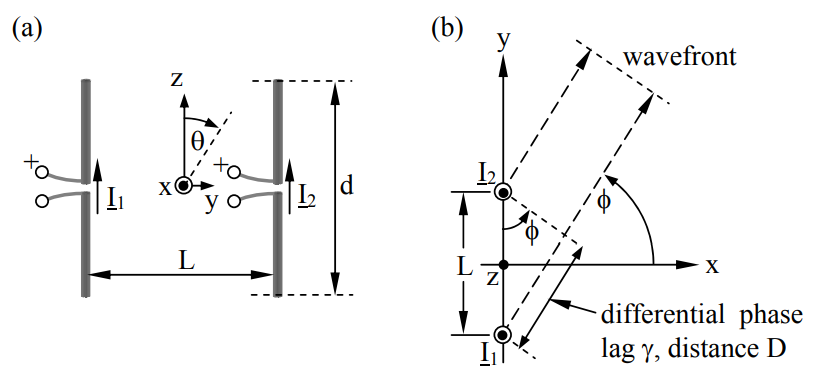
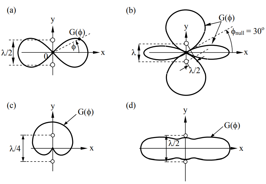
The radiated power P(r,ϕ) in Figure 10.4.1 depends on the differential phase lag γ between the contributions from the two antennas. When the two dipoles are excited equally (I_1=I_2=I_) and are spaced L = λ/2 apart, the two rays add in phase everywhere in the x-z plane perpendicular to the array axis, but are λ/2 (180o) out of phase and cancel along the array (y) axis. The resulting G(ϕ) is sketched in Figure 10.4.2(a) for the x-y plane. If L = λ as illustrated in Figure 10.4.2(b), then the two rays add in phase along both the x-z plane and the y axis, but cancel in the x-y plane at ϕnull =30∘ where the differential delay between the two rays is λ/2, as suggested by the right triangle in the figure.
Figure 10.4.2(c) illustrates how a non-symmetric pattern can be synthesized by exciting the two dipoles out of phase. In this case the lower dipole leads the upper dipole by 90 degrees, so that the total phase difference between the two rays propagating in the negative y direction is 180 degrees, producing cancellation; this phase difference is zero degrees for radiation in the +y direction, so the two rays add. Along the ±x axis the two rays are 90 degrees out of phase so the total E is √2 greater than from a single dipole, and the intensity is doubled. When the two phasors are in phase the total E is doubled and the radiated intensity is 4 times that of a single dipole; thus the intensity radiated along the ±x axis is half that radiated along the +y axis. Figure 10.4.2(d) illustrates how a null-free pattern can be synthesized with non-equal excitation of the two dipoles. In this case the two dipoles are driven in phase so that the radiated phase difference is 180 degrees along the ±y axis due to the λ/2 separation of the dipoles. Nulls are avoided by exciting either dipole with a current that is ~40 percent of the other so that the ratio of maximum gain to minimum gain is ~[(1 + 0.4)/(1 - 0.4)]2 = 5.44, and the pattern is vaguely rectangular.
A mathematical expression for the gain pattern can also be derived. Superimposing (10.2.8) for I_1 and I_2 yields:
→E_ff≅ˆθj(kηodeff/4πr)sinθ(I_1e−jkr1+I_2e−jkr2)≅ˆθj(ηodeff/2λr)sinθ I_ e−jkr(e+0.5jkLsinϕ+e−0.5jkLsinϕ)≅ˆθj(ηoI_deff/λr)sinθe−jkrcos(πLλ−1sinϕ)
where we have used the identities ejα+e−jα=2cosα and k=2π/λ.
If the two dipoles of Figure 10.4.1 are fed in phase and their separation is L = 2λ, at what angles ϕ in the x-y plane are there nulls and peaks in the gain G(ϕ)? Are these peaks equal? Repeat this analysis for L = λ/4, assuming the voltage driving the dipole at y > 0 has a 90° phase lag relative to the other dipole.
Solution
Referring to Figure 10.4.1, there are nulls when the phase difference γ between the two rays arriving at the receiver is π or 3π, or equivalently, D = λ/2 or 3λ/2, respectively. This happens at the angles ϕ=±sin−1(D/L)=±sin−1[(λ/2)/2λ]=±sin−1(0.25)≅±14∘, and ϕ=±sin−1(0.75)≅±49∘. There are also nulls, by symmetry, at angles 180° away, or at ϕ ≅ ±194° and ±229°. There are gain peaks when the two rays are in phase (ϕ = 0° and 180°) and when they differ in phase by 2π or 4π, which happens when ϕ=±sin−1(λ/2λ)=±30∘ and ϕ = ±210°, or when ϕ = ±90°, respectively. The gain peaks are equal because they all correspond to the two rays adding coherently with the same magnitudes. When L = λ/4 the two rays add in phase at ϕ = 90° along the +y axis because in that direction the phase lag balances the 90° delay suffered by the ray from the dipole on the -y axis. At ϕ = 270° these two 90-degree delays add rather than cancel, so the two rays cancel in that direction, producing a perfect null.
Array antennas with mirrors
One of the simplest ways to boost the gain of a short dipole antenna is to place a mirror behind it to as to reinforce the radiation in the desired forward direction and cancel it behind. Figure 10.4.3 illustrates how a short current element I placed near a perfectly conducting planar surface will behave as if the mirror were replaced by an image current an equal distance behind the mirror and pointed in the opposite direction parallel to the mirror but in the same direction normal to the mirror. The fields in front of the mirror are identical with and without the mirror if it is sufficiently large. Behind the mirror the fields approach zero, of course. Image currents and charges were discussed in Section 4.2.
Figure 10.4.3(a) illustrates a common way to boost the forward gain of a dipole antenna by placing it λ/4 in front of a planar mirror and parallel to it.
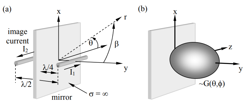
The image current is 180 degrees out of phase, so the λ/2 delay suffered by the image ray brings it into phase coherence with the direct ray, effectively doubling the far field Eff and quadrupling the intensity and gain Go relative to the absence of the mirror. In all directions more nearly parallel to the mirror the source and image are more nearly out of phase, so the gain in those directions is diminished relative to the absence of the mirror. The resulting antenna gain G(θ,ϕ) is sketched in Figure 10.4.3(b), and has no backlobes.
For the case where the dipole current I_2=−I_1 and kr1=kr−(π/2)cosβ, the far-field in the forward direction is the sum of the contributions from I_1 and I_2, as given by (10.4.1):
→E_ff=ˆθ(jηodeff/2λr)sinθ(I_1e−jkr1+I_2e−jkr2)=ˆθ(jηodeff/2λr)sinθe−jkrI_1(ej(π/2)cosβ−e−j(π/2)cosβ)=−ˆθ(ηodeff/λr)sinθe−jkrI _1sin[(π/2)cosβ]
This expression reveals that the antenna pattern has no sidelobes and is pinched somewhat more in the θ direction than in the β direction (these directions are not orthogonal). An on-axis observer will receive a z-polarized signal.
Mirrors can also be parabolic and focus energy at infinity, as discussed further in Section 11.1. The sidelobe-free properties of this dipole-plus-mirror make it a good antenna feed for radiating energy toward much larger parabolic reflectors.
Automobile antennas often are thin metal rods ~1-meter long positioned perpendicular to an approximately flat metal surface on the car; the rod and flat surface are electrically insulated from each other. The rod is commonly fed by a coaxial cable, the center conductor being attached to the base of the rod and the sheath being attached to the adjacent car body. Approximately what is the radiation resistance and pattern in the 1-MHz radio broadcast band, assuming the flat plate is infinite?
Solution
Figure 4.2.3 shows how the image of a current flowing perpendicular to a conducting plane flows in the same direction as the original current, so any current flowing in the rod has an image current that effectively doubles the length of this antenna. The wavelength at 1 MHz is ~300 meters, much longer than the antenna, so the shortdipole approximation applies and the current distribution on the rod and its image resembles that of Figure 10.2.3; thus deff ≅ 1 meter and the pattern above the metal plane is the top half of that illustrated in Figure 10.2.4. The radiation resistance of a normal short dipole antenna (10.3.16) is Rr=2PT/|Io|2=2ηoπ(deff/λ)2/3=0.0088 ohms for deff = 1 meter. Here, however, the total power radiated PT is half that radiated by a short dipole of length 2 meters because there is no power radiated below the conducting plane, so Rr = 0.0044 ohms. The finite size of an automobile effectively warps and shortens both the image current and the effective length of the dipole, although the antenna pattern for a straight current is always dipolar above the ground plane.
Element and array factors
The power radiated by dipole arrays depends on the directional characteristics of the individual dipole antennas as well as on their spacing relative to wavelength λ. For example, (10.4.3) can be generalized to N identically oriented but independently positioned and excited dipoles:
→E_ff≅[ˆθjηodeff2λrsinθ][N∑i=1I_ie−jkri]=→ε_(θ,ϕ)F_(θ,ϕ)
The element factor →ε_(θ,ϕ) for the dipole array represents the behavior of a single element, assuming the individual elements are identically oriented. The array factor, F_(θ,ϕ)=∑NiI_ie−jki, represents the effects of the relative strengths and placement of the elements. The distance between the observer and each element i of the array is ri, and the phase lag kri = 2πri/λ.
Consider the element factor in the x-y plane for the two z-oriented dipoles of Figure 10.4.4(a).
This element factor →ε_(θ,ϕ) is constant, independent of ϕ, and has a circular pattern. The total antenna pattern is |→ε_(θ,ϕ)F_(θ,ϕ)|2 where the array factor F_(θ,ϕ) controls the array antenna pattern in the x-y plane for these two dipoles. The resulting antenna pattern |F_(θ,ϕ)|2 in the x-y plane is plotted in Figure 10.4.4(a) and (b) for the special cases L = λ/2 and L = λ, respectively. Both the array and element factors contribute to the pattern for this antenna in the x-z plane, narrowing its beamwidth (not illustrated).
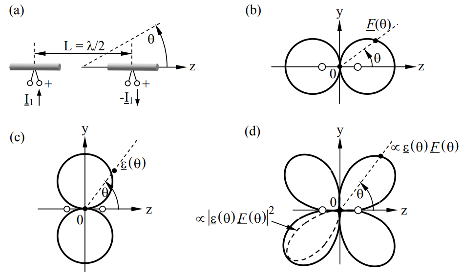
Figure 10.4.4 illustrates a case where both the element and array factors are important; L = λ/2 here and the dipoles are fed 180o out of phase. In this case the out-of-phase signals from the two dipoles cancel everywhere in the x-y plane and add in phase along the z axis, corresponding to the array factor plotted in Figure 10.4.4(b) for the y-z plane. Note that when θ = 60o the two phasors are 45o out of phase and |F_(θ,ϕ)|2 has half its peak value. The element factor in the y-z plane appears in Figure 10.4.4(c), and the dashed antenna pattern |ε_(θ)F_(θ)|2∝G(θ) in Figure 10.4.4(d) shows the effects of both factors (only one of the four lobes is plotted). This antenna pattern is a figure of revolution about the z axis and resembles two wide rounded cones facing in opposite directions.
What are the element and array factors for the two-dipole array for the first part of Example 10.4A?
Solution
From (10.4.5) the element factor for such dipoles is ˆθj(ηodeff/2λr)sinθ. The last factor of (10.4.5) is the array factor for such two-dipole arrays:
F_(θ,ϕ)=I_(e+0.5(j2π2λ/λ)sinϕ+e−0.5(j2π2λ/λ)sinϕ)=(e2πjsinϕ+e−2πjsinϕ)=2I_cos(2πsinϕ)
Uniform dipole arrays
Uniform dipole arrays consist of N identical dipole antennas equally spaced in a straight line. Their current excitation I_1 has equal magnitudes for all i, and a phase angle that uniformly increases by ψ radians between adjacent dipoles. The fields radiated by the array can be determined using (10.4.5):
→E_ff≅[ˆθj(ηodeff/2λr)sinθ][N∑i=1I_ie−jkri]=→ε_(θ,ϕ)F_(θ,ϕ)
The z axis is defined by the orientation of the dipoles, which are all parallel to it. The simplest arrangement of the dipoles is along that same z axis, as in Figure 10.4.5, although (10.4.6) applies equally well if the dipoles are spaced in any arbitrary direction. Figure 10.4.1(a) illustrates the alternate case where two dipoles are spaced along the y axis, and Figure 10.4.2 shows the effects on the patterns.
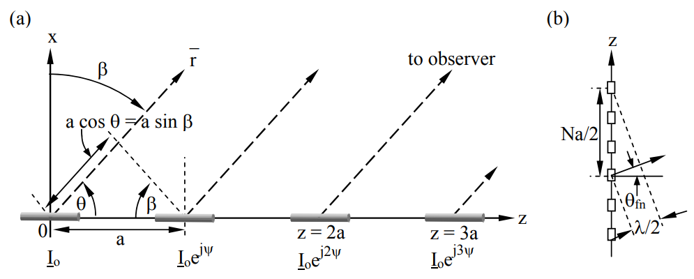
Consider the N-element array for Figure 10.4.5(a). The principal difference between these two-dipole cases and N-element uniform arrays lies in the array factor:
F_(θ,ϕ)=N∑i=1I_ie−jkri=I_0e−jkrN−1∑i=0ejiψejjkacosθ=I_0e−jkrN−1∑i=0[ej(ψ+kacosθ)]i
The geometry illustrated in Figure 10.4.5(a) yields a phase difference of (ψ + ka cosθ) between the contributions from adjacent dipoles.
Using the two identities:
N−1∑i=0xi=(1−xN)/(1−x)
1−ejA=ejA/2(e−jA/2−e+jA/2)=−2jejA/2sin(A/2)
(10.4.7) becomes:
F_(θ,ϕ)=I_0e−jkr1−ejN(ψ+kacosθ)1−ej(ψ+kacosθ)=I_0e−jkr×ejN(ψ+kacosθ)/2ej(ψ+kacosθ)/2sin[N(ψ+kacosθ)/2]sin[(ψ+kacosθ)/2]
Since the element factor is independent of ϕ, the antenna gain has the form:
G(θ)∝|F_(θ,ϕ)|2∝sin2[N(ψ+kacosθ)/2]sin2[(ψ+kacosθ)/2]
If the elements are excited in phase (ψ = 0), then the maximum gain is broadside with θ = 900, because only in that direction do all N rays add in perfect phase. In this case the first nulls θfirst null bounding the main beam occur when the numerator of (10.4.11) is zero, which happens when:
N2kacosθfirst null =±π
Note that the factor ka = 2πa/λ is in units of radians, and therefore cosθfirst null =±λ/Na. If θfirst null ≡π/2±θfn where θfn is the null angle measured from the x-y plane rather than from the z axis, then we have cosθfirst null =sinθfn≅θfn and:
θfn≅±λ/Na [ radians ]
The following simple geometric argument yields the same answer. Figure 10.4.5(b) shows that the first null of this 6-dipole array occurs when the rays from the first and fourth dipole element cancel, for then the rays from the second and fifth, and the third and sixth will also cancel. This total cancellation occurs when the delay between the first and fourth ray is λ/2, which corresponds to the angle θfn=±sin−1[(λ/2)/(aN/2)]≅±λ/aN.
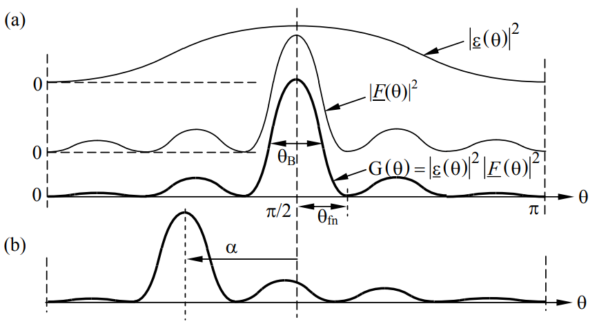
The angle θfn between the beam axis and the first null is approximately the half-power beamwidth θB of an N-element antenna array. The antenna gain G(θ) associated with (10.4.11) for N = 6, ψ = 0, and a = λ/2 is sketched in Figure 10.4.6(a), together with the squares of the array factor [from (10.4.10)] and element factor [from (10.4.6)]. In this case θfn=±sin−1(2/N)≅±2/N radians ≅θB.
If ψ ≠ 0 so that the excitation phase varies linearly across the array, then the main beam and the rest of the pattern is “squinted” or “scanned” to one side by angle α. Since a phase delay of ψ is equivalent to a path delay of δ, where ψ = kδ, and since the distance between adjacent dipoles is a, it follows that adjacent rays for a scanned beam will be in phase at angle θ=π/2+sin−1(δ/a)=π/2+α, where:
α=sin−1(δ/a)=sin−1(ψλ/2πa)( scan angle )
as sketched in Figure 10.4.6(b) for the case ψ = 2 radians, a = λ/2, and α ≅ 40o.
Note that larger element separations a can produce multiple main lobes separated by smaller ones. Additional main lobes appear when the argument (ψ + ka cosθ)/2 in the denominator of (10.4.11) is an integral multiple of π so that the denominator is zero; the numerator is zero at the same angles, so the ratio is finite although large. To preclude multiple main lobes the spacing should be a < λ, or even a < λ/2 if the array is scanned.
A uniform row of 100 x-oriented dipole antennas lies along the z axis with inter-dipole spacing a = 2λ. At what angles θ in the y-z plane is the gain maximum? See Figure 10.4.5 for the geometry, but note that the dipoles for our problem are x-oriented rather than z-oriented. What is the angle δ between the two nulls adjacent to θ ≅ π/2? What is the gain difference δG(dB) between the main lobe at θ = π/2 and its immediately adjacent sidelobes? What difference in excitation phase ψ between adjacent dipoles is required to scan these main lobes 10° to one side?
Solution
The gain is maximum when the rays from adjacent dipoles add in phase, and therefore all rays add in phase. This occurs at θ = 0, ± π/2 , and ±sin−1 (λ/a) ≅ 30° [see Figure 10.4.5(b) for the approximate geometry, where we want a phase lag of λ to achieve a gain maximum]. The nulls nearest θ = π/2 occur at that θfn when the rays from the first and 51st dipoles first cancel [see text after (10.4.13)], or when θfn=π2±sin−1(λ/2aN/2)=π2±sin−1(λ/22λN/2)≅π2±12N; thus δ = 1/N radians ≅ 0.57o. The array factors for this problem and Figure 10.4.5(a) are the same, so (10.4.10) applies. Near θ ≅ π/2 the element factor is approximately constant and can therefore be ignored because we seek only gain ratios. We define β≡π/2 − θ so cos θ becomes sin β. Therefore (10.4.11) becomes Go(θ)∝|F(θ,ϕ)|2∝sin2(Nkλsinβ)/sin2(kλsinβ) where ψ=0. β<<1, so sinβ≅β. Similarly, kλβ<<1 so sin(kλβ)≅kλβ. Thus Go(β=0)∝∼(Nkλβ)2/(kλβ)2=N2, and the first adjacent peak in gain occurs when Nkλsinβfirst peak =1, so G(β=βfirst peak )∝∼(kλβfirst peak )−2. The numerator is unity when Nkλβfirst peak ≅3π/2, or βfirst peak ≅3π/2Nkλ=3/(4N). Therefore G(β=βfirst peak )∝∼(2π3/4N)−2≅0.045N2, which is 10log10(0.045)=−13.5 dB relative to the peak N2. A 10° scan angle requires the rays from adjacent dipoles to be in phase at that angle, and therefore the physical lag δ meters between the two rays must satisfy sinβscan=δ/a=δ/2λ. The corresponding phase lag in the leading dipole is ψ=kδ=(2π/λ)(2λsinβscan)=4πsin(10∘)radians=125∘.
Phasor addition in array antennas
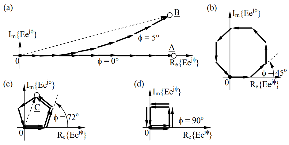
Phasor addition can be a useful tool for analyzing antennas. Consider the linear dipole array of Figure 10.4.5, which consists of N identical z-oriented dipole antennas spaced at distance a equally along the z-axis. In direction θ from the z axis the array factor is the sum of the phasors emitted from each dipole. Figure 10.4.6(a) shows this sum A_ for the x-y plane (θ = 90°) when the dipoles are all excited in phase and N = 8. This yields the maximum possible gain for this antenna. As θ departs from 90° (broadside radiation) the phasors each rotate differently and add to form a progressively smaller sum B_. When the total phasor B_ corresponds to δϕ = 5-degree lag for each successive contribution, then θ=cos−1(5360λa). Figure 10.4.6(b, c, and d) show the sum B_ when δϕ is 45°, 72°, and 90°, respectively. The antenna gain is proportional to |B_|2. Figures (b) and (d) correspond to radiation angles θ that yield nulls in the pattern (|B_|=0), while (c) is near a local maximum in the antenna pattern. Because ∣C_∣ is ∼0.2|A_|, the gain of this sidelobe is ~0.04 times the maximum gain (|C_|2≅0.04|A_|2), or ~14 dB weaker.54 The spatial angles θ corresponding to (a) - (d) depend on the inter-dipole distance 'a'.
If a = 2λ, then angles θ from the z axis that correspond to phasor A_ in Figure 10.4.7 (a) are 0°, 60°, 90°, 120°, and 180°; the peaks at 0 and 180° fall on the null of the element factor and can be ignored. The angle from the array axis is θ, and 'a' is the element spacing, as illustrated in Figure 10.4.5. The angles θ = 0° and 180° correspond to cos−1(2λ/2λ), , while θ = 60° and θ = 120° correspond to cos−1(λ/2λ), and θ = 90° corresponds to cos−1(0/2λ); the numerator in the argument of cos-1 is the lag distance in direction θ, and the denominator is the element spacing 'a'. Thus this antenna has three equal peaks in gain: θ = 60, 90, and 120°, together with numerous smaller sidelobes between those peaks.
54 dB ≡ 10 log10N, so N = 0.04 corresponds to ~-14 dB.
Four small sidelobes occur between the adjacent peaks at 60°, 90°, and 120°. The first sidelobe occurs in each case for ϕ ≅ 70° as illustrated in Figure 10.4.2(c), i.e., approximately half-way between the nulls at ϕ = 45° [Figure 10.4.2(b)] and ϕ = 90° [Figure 10.4.2(d)], and the second sidelobe occurs for ϕ ≅ 135°, between the nulls for ϕ = 90° [Figure 10.4.2(d)] and ϕ = 180° (not illustrated). Consider, for example, the broadside main lobe at θ = 90°; for this case ϕ = 0°. As θ decreases from 90° toward zero, ϕ increases toward 45°, where the first null occurs as shown in (b); the corresponding θnull =cos−1[(ϕλ/360)/2λ]=86.4∘. The denominator 2λ in the argument is again the inter-element spacing. The first sidelobe occurs when ϕ ≅ 72° as shown in (c), and θ≅cos−1[(ϕλ/360)/2λ]=84.4∘. The next null occurs at ϕ = 90° as shown in (d), and θnull =cos−1[(ϕλ/360)/2λ]=82.8∘. The second sidelobe occurs for ϕ ≅ 135°, followed by a null when ϕ = 180°. The third and fourth sidelobes occur for ϕ ≅ 225° and 290° as the phasor patterns repeat in reverse sequence: (d) is followed by (c) and then (b) and (a) as θ continues to decline toward the second main lobe at θ = 60°. The entire gain pattern thus has three major peaks at 60, 90, and 120°, typically separated by four smaller sidelobes intervening between each major pair, and also grouped near θ = 0° and 180°.
What is the gain GS of the first sidelobe of an n-element linear dipole array relative to the main lobe Go as n → ∞?
Solution
Referring to Figure 10.4.7(c), we see that as n→∞ the first sidelobe has an electric field EffS that is the diameter of the circle formed by the n phasors when ∑ni=1|E_i|=Effo is ~1.5 times the circumference of that circle, or . The ratio of the gains is therefore GS/Go=|Effs/Effo|2=(1/1.5π)2=0.045, or -13.5 dB.
Multi-beam antenna arrays
Some antenna arrays are connected so as to produce several independent beams oriented in different directions simultaneously; phased array radar antennas and cellular telephone base stations are common examples. When multiple antennas are used for reception, each can be filtered and amplified before they are added in as many different ways as desired. Sometimes these combinations are predetermined and fixed, and sometimes they are adjusted in real time to place nulls on sources of interference or to place maxima on transmitters of interest, or to do both.
The following cellular telephone example illustrates some of the design issues. The driving issue here is the serious limit to network capacity imposed by the limited bandwidth available at frequencies suitable for urban environments. The much broader spectrum available in the centimeter and millimeter-wave bands propagates primarily line-of-sight and is not very useful for mobile applications; lower frequencies that diffract well are used instead, although the available bandwidth is less. The solution is to reuse the same low frequencies multiple times, even within the same small geographic area. This is accomplished using array antennas that can have multiple inputs and outputs.
A typical face of a cellular base station antenna has 3 or 4 elements that radiate only into the forward half-space. They might also have a combining circuit that forms two or more desired beams. An alternate way to use these arrays based on switching is described later. Three such faces, such as those illustrated in Figure 10.4.8(a) with four elements spaced at 3λ, might be arranged in a triangle and produce two sets of antenna lobes, for example, the ϕ = 0 set and the ϕ = π set indicated in (b) by filled and dashed lines, respectively.
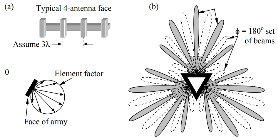
As before, ϕ is the phase angle difference introduced between adjacent antenna elements. Interantenna separations of 3λ result in only 5 main lobes per face, because the two peaks in the plane of each face are approximately zero for typical element factors. Between each pair of peaks there are two small sidelobes, approximately 14 dB weaker as shown above.
These two sets (ϕ = 0, ϕ = π) can share the same frequencies because digital communication techniques can tolerate overlapping signals if one is more than ~10-dB weaker. Since each face of the antenna can be connected simultaneously to two independent receivers and two independent transmitters, as many as six calls could simultaneously use the same frequency band, two per face. A single face would not normally simultaneously transmit and receive the same frequency, however. The lobe positions can also be scanned in angle by varying ϕ so as to fill any nulls. Designing such antennas to maximize frequency reuse requires care and should be tailored to the distribution of users within the local environment. In unobstructed environments there is no strong limit to the number of elements and independent beams that can be used per face, or to the degree of frequency reuse. Moreover, half the beams could be polarized one way, say right-circular or horizontal, and the other half could be polarized with the orthogonal polarization, thereby doubling again the number of possible users of the same frequencies. Polarization diversity works poorly for cellular phones, however, because users orient their dipole antennas as they wish.
In practice, most urban cellular towers do not currently phase their antennas as shown above because many environments suffer from severe multipath effects where reflected versions of the same signals arrive at the receiving tower from many angles with varying delays. The result is that at each antenna element the phasors arriving from different directions with different phases and amplitudes will add to produce a net signal amplitude that can be large or small. As a result one of the elements facing a particular direction may have a signal-to-interference ratio that is more than 10 dB stronger than another for this reason alone, even though the antenna elements are only a few wavelengths away in an obstacle-free local environment. Signals have different differential delays at different frequencies and therefore their peak summed values at each antenna element are frequency dependent. The antenna-use strategy in this case is to assign users to frequencies and single elements that are observed to be strong for that user, so that another user could be overlaid on the same frequency while using a different antenna element pointed in the same direction. The same frequency-reuse strategy also works when transmitting because of reciprocity.
That signal strengths are frequency dependent in multipath environments is easily seen by considering an antenna receiving both the direct line-of-sight signal with delay t1 and a reflected second signal with comparable strength and delay t2. If the differential lag c(t2 - t1) = nλ = D for integer n, then the two signals will add in phase and reinforce each other. If the lag D = (2n + 1)λ/2, then they will partially or completely cancel. If D = 10λ and the frequency f increases by 10 percent, then the lag measured in wavelengths will also change 10 percent as the sum makes a full peak-to-peak cycle with a null between. Thus the gap between frequency nulls is ~δf = f(λ/D) = c/D Hz. The depth of the null depends on the relative magnitudes of the two rays that interfere. As the number of rays increases the frequency structure becomes more complex. This phenomenon of signals fading in frequency and time as paths and frequencies change is called multipath fading.