2.10: Variable Separation – Cylindrical Coordinates

Now, let us discuss whether it is possible to generalize our approach to problems whose geometry is still axially-symmetric, but with a substantial dependence of the potential on the axial coordinate (\(\ \partial \phi / \partial z \neq 0\)). The classical example of such a problem is shown in Fig. 17. Here the sidewall and the bottom lid of a hollow round cylinder are kept at a fixed potential (say, \(\ \phi=0\)), but the potential \(\ V\) fixed at the top lid is different. Evidently, this problem is qualitatively similar to the rectangular box problem solved above (Fig. 13), and we will also try to solve it first for the case of arbitrary voltage distribution over the top lid: \(\ V=V(\rho, \varphi)\).

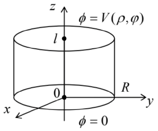Fig. 2.17. A cylindrical volume with conducting walls.

Following the main idea of the variable separation method, let us require that each partial function \(\ \phi_{k}\) in Eq. (84) satisfies the Laplace equation, now in the full cylindrical coordinates \(\ \{\rho, \varphi, z\}\):³⁹

\[\ \frac{1}{\rho} \frac{\partial}{\partial \rho}\left(\rho \frac{\partial \phi_{k}}{\partial \rho}\right)+\frac{1}{\rho^{2}} \frac{\partial^{2} \phi_{k}}{\partial \varphi^{2}}+\frac{\partial^{2} \phi_{k}}{\partial z^{2}}=0.\tag{2.124}\]

Plugging in \(\ \phi_{k}\) in the form of the product \(\ \mathcal{R}(\rho) \mathcal{F}(\varphi) \mathcal{Z}(z)\) into Eq. (124) and dividing all resulting terms by \(\ \mathcal{RFZ}\), we get

\[\ \frac{1}{\rho \mathcal{R}} \frac{d}{d \rho}\left(\rho \frac{d \mathcal{R}}{d \rho}\right)+\frac{1}{\rho^{2} \mathcal{F}} \frac{d^{2} \mathcal{F}}{d \varphi^{2}}+\frac{1}{\mathcal{Z}} \frac{d^{2} \mathcal{Z}}{d z^{2}}=0.\tag{2.125}\]

Since the first two terms of Eq. (125) can only depend on the polar variables \(\ \rho\) and \(\ \varphi\), while the third term, only on \(\ z\), at least that term should equal a constant. Denoting it (just like in the rectangular box problem) by \(\ \gamma^{2}\), we get the following set of two equations:

\[\ \frac{d^{2} \mathcal{Z}}{d z^{2}}=\gamma^{2} z,\tag{2.126}\]

\[\ \frac{1}{\rho \mathcal{R}} \frac{d}{d \rho}\left(\rho \frac{d \mathcal{R}}{d \rho}\right)+\gamma^{2}+\frac{1}{\rho^{2} \mathcal{F}} \frac{d^{2} \mathcal{F}}{d \varphi^{2}}=0.\tag{2.127}\]

Now, multiplying all the terms of Eq. (127) by \(\ \rho^{2}\), we see that the last term of the result, \(\ \left(d^{2} \mathcal{F} /d \varphi^{2}\right) / \mathcal{F}\), may depend only on \(\ \varphi\), and thus should be constant. Calling that constant \(\ v^{2}\) (just as in Sec. 6 above), we separate Eq. (127) into an angular equation,

\[\ \frac{d^{2} \mathcal{F}}{d \varphi^{2}}+v^{2} \mathcal{F}=0,\tag{2.128}\]

and a radial equation:

\[\ \frac{d^{2} \mathcal{R}}{d \rho^{2}}+\frac{1}{\rho} \frac{d \mathcal{R}}{d \rho}+\left(\gamma^{2}-\frac{v^{2}}{\rho^{2}}\right) \mathcal{R}=0.\tag{2.129}\]

We see that the ordinary differential equations for the functions \(\ \mathcal{Z}(z)\) and \(\ \mathcal{F}(\varphi)\) (and hence their solutions) are identical to those discussed earlier in this chapter. However, Eq. (129) for the radial function \(\ \mathcal{R}(\rho)\) (called the Bessel equation) is more complex than in the 2D case, and depends on two
independent constant parameters, \(\ \gamma\) and \(\ v\). The latter challenge may be readily overcome if we notice that any change of \(\ \gamma\) may be reduced to the corresponding re-scaling of the radial coordinate \(\ \rho\). Indeed, introducing a dimensionless variable \(\ \xi \equiv \gamma \rho\),⁴⁰ Eq. (129) may be reduced to an equation with just one parameter, \(\ v\).

Bessel equation

\[\ \frac{d^{2} \mathcal{R}}{d \xi^{2}}+\frac{1}{\xi} \frac{d \mathcal{R}}{d \xi}+\left(1-\frac{v^{2}}{\xi^{2}}\right) \mathcal{R}=0.\tag{2.130}\]

Moreover, we already know that for angle-periodic problems, the spectrum of eigenvalues of Eq. (128) is discrete: \(\ v=n\), with integer \(\ n\).

Unfortunately, even in this case, Eq. (130), which is the canonical form of the Bessel equation, cannot be satisfied by a single “elementary” function. Its solutions that we need for our current problem are called the Bessel function of the first kind, of order \(\ v\), commonly denoted as \(\ J_v(\xi)\). Let me review in brief those properties of these functions that are most relevant for our problem – and many other problems discussed in this series.⁴¹

First of all, the Bessel function of a negative integer order is very simply related to that with the positive order:

\[\ J_{-n}(\xi)=(-1)^{n} J_{n}(\xi),\tag{2.131}\]

enabling us to limit our discussion to the functions with \(\ n \geq 0\). Figure 18 shows four of these functions with the lowest positive \(\ n\).

Fig. 2.18. Several Bessel functions \(\ J_{n}(\xi)\) of integer order. The dashed lines show the envelope of the asymptotes (135).

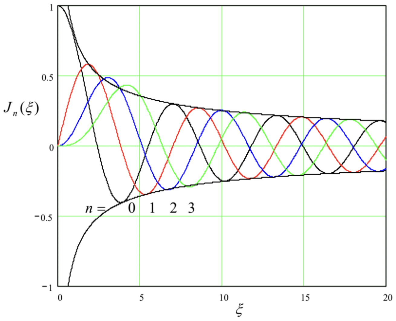
As its argument is increased, each function is initially close to a power law: \(\ J_{0}(\xi) \approx 1\), \(\ J_{1}(\xi) \approx \xi / 2=\xi/2\), \(\ J_{2}(\xi) \approx \xi^{2} / 8\), etc. This behavior follows from the Taylor series

\[\ J_{n}(\xi)=\left(\frac{\xi}{2}\right)^{n} \sum_{k=0}^{\infty} \frac{(-1)^{k}}{k !(n+k) !}\left(\frac{\xi}{2}\right)^{2 k},\tag{2.132}\]

which is formally valid for any \(\ \xi\), and may even serve as an alternative definition of the functions \(\ J_{n}(\xi)\). However, the series is converging fast only at small arguments, \(\ \xi<n\), where its leading term is

\[\ \left.J_{n}(\xi)\right|_{\xi \rightarrow 0} \rightarrow \frac{1}{n !}\left(\frac{\xi}{2}\right)^{n}.\tag{2.133}\]

At \(\ \xi \approx n+1.86 n^{1 / 3}\), the Bessel function reaches its maximum⁴²

\[\ \max _{\xi}\left[J_{n}(\xi)\right] \approx \frac{0.675}{n^{1 / 3}},\tag{2.134}\]

and then starts to oscillate with a period gradually approaching 2 \(\ \pi\), a phase shift that increases by \(\ \pi / 2\) with each unit increment of \(\ n\), and an amplitude that decreases as \(\ \xi^{1 / 2}\). All these features are described by the following asymptotic formula:

\[\ \left.J_{n}(\xi)\right|_{\xi \rightarrow \infty} \rightarrow\left(\frac{2}{\pi \xi}\right)^{1 / 2} \cos \left(\xi-\frac{\pi}{4}-\frac{n \pi}{2}\right),\tag{2.135}\]

which starts to give a reasonable approximation very soon after the function peaks – see Fig. 18.⁴³

Now we are ready for our case study (Fig. 17). Let us select functions the \(\ \mathcal{Z}(z)\) so that they satisfy Eq. (126) and the bottom-lid boundary condition \(\ \mathcal{Z}(0)=0\), i.e. are proportional to \(\ \sinh \gamma z\) – cf. Eq. (94). Then we get

\[\ \phi=\sum_{n=0}^{\infty} \sum_{\gamma} J_{n}(\gamma \rho)\left(c_{n \gamma} \cos n \varphi+s_{n \gamma} \sin n \varphi\right) \sinh \gamma z.\tag{2.136}\]

Next, we need to satisfy the zero boundary condition at the cylinder’s side wall \(\ (\rho=R)\). This may be ensured by taking

\[\ J_{n}(\gamma R)=0.\tag{2.137}\]

Since each function \(\ J_{n}(x)\) has an infinite number of positive zeros (see Fig. 18 again), which may be numbered by an integer index \(\ m=1,2, \ldots\), Eq. (137) may be satisfied with an infinite number of discrete values of the separation parameter \(\ \gamma\).

\[\ \gamma_{n m}=\frac{\xi_{n m}}{R},\tag{2.138}\]

where \(\ \xi_{n m}\) is the \(\ m\)-th zero of the function \(\ J_{n}(x)\) – see the top numbers in the cells of Table 1. (Very soon we will see what do we need the bottom numbers for.)

Table 2.1. Approximate values of a few first zeros, \(\ \xi_{n m}\), of a few lowest-order Bessel functions \(\ J_{n}(\xi)\) (the top number in each cell), and the values of \(\ d J_{n}(\xi) / d \xi\) at these points (the bottom number).

	\(\ m = 1\)	2	3	4	5	6
\(\ n = 0\)	2.40482 -0.51914	5.52008 +0.34026	8.65372 -0.27145	11.79215 +0.23245	14.93091 -0.20654	18.07106 +0.18773
1	3.83171 -0.40276	7.01559 +0.30012	10.17347 -0.24970	13.32369 +0.21836	16.47063 -0.19647	19.61586 +0.18006
2	5.13562 -0.33967	8.41724 +0.27138	11.61984 -0.23244	14.79595 +0.20654	17.95982 -0.18773	21.11700 +0.17326
3	6.38016 -0.29827	9.76102 +0.24942	13.01520 -0.21828	16.22347 +0.19644	19.40942 -0.18005	22.58273 +0.16718
4	7.58834 -0.26836	11.06471 +0.23188	14.37254 -0.20636	17.61597 +0.18766	20.82693 -0.17323	24.01902 +0.16168
5	8.77148 -0.24543	12.33860 +0.21743	15.70017 -0.19615	18.98013 +0.17993	22.21780 -0.16712	25.43034 +0.15669

Hence, Eq. (136) may be represented in a more explicit form:

Variable separation in cylindrical coordinates (example)

\[\ \phi(\rho, \varphi, z)=\sum_{n=0}^{\infty} \sum_{m=1}^{\infty} J_{n}\left(\xi_{n m} \frac{\rho}{R}\right)\left(c_{n m} \cos n \varphi+s_{n m} \sin n \varphi\right) \sinh \left(\xi_{n m} \frac{z}{R}\right).\tag{2.139}\]

Here the coefficients \(\ c_{n m}\) and \(\ s_{n m}\) have to be selected to satisfy the only remaining boundary condition – that on the top lid:

\[\ \phi(\rho, \varphi, l) \equiv \sum_{n=0}^{\infty} \sum_{m=1}^{\infty} J_{n}\left(\xi_{n m} \frac{\rho}{R}\right)\left(c_{n m} \cos n \varphi+s_{n m} \sin n \varphi\right) \sinh \left(\xi_{n m} \frac{l}{R}\right)=V(\rho, \varphi).\tag{2.140}\]

To use it, let us multiply both parts of Eq. (140) by \(\ J_{n}\left(\xi_{n m^{\prime}} \rho / R\right) \cos n^{\prime} \varphi\), integrate the result over the lid area, and use the following property of the Bessel functions:

\[\ \int_{0}^{1} J_{n}\left(\xi_{n m} s\right) J_{n}\left(\xi_{n m^{\prime}} s\right) s d s=\frac{1}{2}\left[J_{n+1}\left(\xi_{n m}\right)\right]^{2} \delta_{m m^{\prime}}.\tag{2.141}\]

The last relation expresses a very specific (“2D”) orthogonality of the Bessel functions with different indices \(\ m\) do not confuse them with the function orders \(\ n\), please!⁴⁴ Since it relates two Bessel functions of the same order \(\ n\), it is natural to ask why its right-hand side contains the function with a different order \(\ (n+1)\). Some gut feeling of that may come from one more very important property of the Bessel functions, the so-called recurrence relations:⁴⁵

\[\ J_{n-1}(\xi)+J_{n+1}(\xi)=\frac{2 n J_{n}(\xi)}{\xi},\tag{2.142a}\]

\[\ J_{n-1}(\xi)-J_{n+1}(\xi)=2 \frac{d J_{n}(\xi)}{d \xi},\tag{2.142b}\]

which in particular yield the following formula (convenient for working out some Bessel function integrals):

\[\ \frac{d}{d \xi}\left[\xi^{n} J_{n}(\xi)\right]=\xi^{n} J_{n-1}(\xi).\tag{2.143}\]

For our current purposes, let us apply the recurrence relations at the special points \(\ \xi_{n m}\). At these points, \(\ J_{n}\) vanishes, and the system of two equations (142) may be readily solved to get, in particular,

\[\ J_{n+1}\left(\xi_{n m}\right)=-\frac{d J_{n}}{d \xi}\left(\xi_{n m}\right),\tag{2.144}\]

so that the square bracket on the right-hand side of Eq. (141) is just \(\ \left(d J_{n} / d \xi\right)^{2}\) at \(\ \xi=\xi_{n m}\). Thus the values of the Bessel function derivatives at the zero points of the function, given by the lower numbers in the cells of Table 1, are as important for boundary problem solutions as the zeros themselves.

Since the angular functions \(\ \cos n \varphi\) are also orthogonal – both to each other,

\[\ \int_{0}^{2 \pi} \cos (n \varphi) \cos \left(n^{\prime} \varphi\right) d \varphi=\pi \delta_{n n^{\prime}},\tag{2.145}\]

and to all functions \(\ \sin n \varphi\), the integration over the lid area kills all terms of both series in Eq. (140), besides just one term proportional to \(\ c_{n^{\prime} m^{\prime}}\), and hence gives an explicit expression for that coefficient. The counterpart coefficients \(\ s_{n^{\prime} m^{\prime}}\) may be found by repeating the same procedure with the replacement of \(\ \cos n^{\prime} \varphi\) by \(\ \sin n^{\prime} \varphi\). This evaluation (left for the reader’s exercise) completes the solution of our problem for an arbitrary lid potential \(\ V(\rho, \varphi)\).

Still, before leaving the Bessel functions (for a while only :-), we need to address two important issues. First, we have seen that in our cylinder problem (Fig. 17), the set of functions \(\ J_{n}\left(\xi_{n m} \rho / R\right)\) with different indices \(\ m\) (which characterize the degree of Bessel function’s stretch along axis \(\ \rho\)) play the role
similar to that of functions \(\ \sin (\pi n x / a)\) in the rectangular box problem shown in Fig. 13. In this context, what is the analog of functions \(\ \cos (\pi n x / a)\) – which may be important for some boundary problems? In a more formal language, are there any functions of the same argument \(\ \xi \equiv \xi_{n m} \rho / R\), that would be linearly independent of the Bessel functions of the first kind, while satisfying the same Bessel equation (130)?

The answer is yes. For the definition of such functions, we first need to generalize our prior formulas for \(\ J_{n}(\xi)\), and in particular Eq. (132), to the case of arbitrary, not necessarily real order \(\ v\). Mathematics says that the generalization may be performed in the following way:

\[\ J_{v}(\xi)=\left(\frac{\xi}{2}\right)^{v} \sum_{k=0}^{\infty} \frac{(-1)^{k}}{k ! \Gamma(v+k+1)}\left(\frac{\xi}{2}\right)^{2 k},\tag{2.146}\]

where \(\ \Gamma(s)\) is the so-called gamma function that may be defined as⁴⁶

\[\ \Gamma(s) \equiv \int_{0}^{\infty} \xi^{s-1} e^{-\xi} d \xi.\tag{2.147}\]

The simplest, and the most important property of the gamma function is that for integer values of its argument, it gives the factorial of the number smaller by one:

\[\ \Gamma(n+1)=n ! \equiv 1 \cdot 2 \cdot \ldots \cdot n,\tag{2.148}\]

so it is essentially a generalization of the notion of the factorial to all real numbers.

The Bessel functions defined by Eq. (146) satisfy, after the replacements \(\ n \rightarrow v\) and \(\ n ! \rightarrow \Gamma(n+1)\), virtually all the relations discussed above, including the Bessel equation (130), the asymptotic formula (135), the orthogonality condition (141), and the recurrence relations (142). Moreover, it may be shown that \(\ v \neq n\), functions \(\ J_{v}(\xi)\) and \(\ J_{-v}(\xi)\) are linearly independent of each other, and hence their linear combination may be used to represent the general solution of the Bessel equation. Unfortunately, as Eq. (131) shows, for \(\ v=n\) this is not true, and a solution linearly independent of \(\ J_{n}(\xi)\) has to be formed differently. The most common way to do that is first to define, for all \(\ v \neq n\), the following functions:

\[\ Y_{v}(\xi) \equiv \frac{J_{v}(\xi) \cos v \pi-J_{-v}(\xi)}{\sin v \pi},\tag{2.149}\]

called the Bessel functions of the second kind, or more often the Weber functions,⁴⁷ and then to follow the limit \(\ v \rightarrow n\). At this, both the numerator and denominator of the right-hand side of Eq. (149) tend to zero, but their ratio tends to a finite value called \(\ Y_{n}(x)\). It may be shown that the resulting functions are
still the solutions of the Bessel equation and are linearly independent of \(\ J_{n}(x)\), though are related just as those functions if the sign of \(\ n\) changes:

\[\ Y_{-n}(\xi)=(-1)^{n} Y_{n}(\xi).\tag{2.150}\]

Figure 19 shows a few Weber functions of the lowest integer orders.

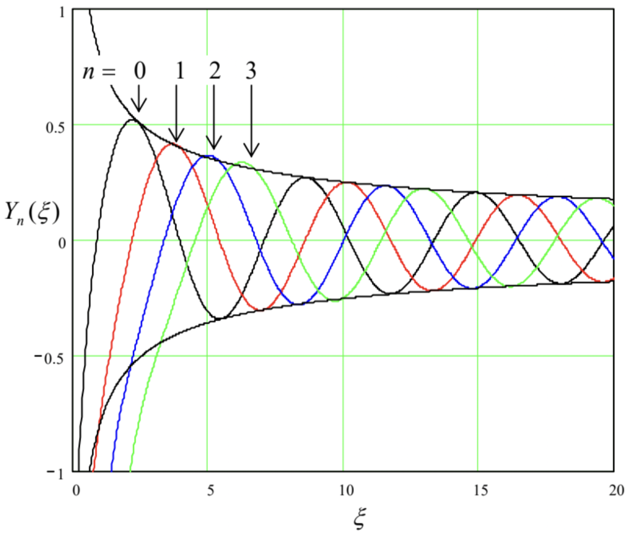Fig. 2.19. A few Bessel functions of the second kind (a.k.a. the Weber functions, a.k.a. the Neumann functions).

The plots show that the asymptotic behavior is very much similar to that of \(\ J_{n}(\xi)\),

\[\ Y_{n}(\xi) \rightarrow\left(\frac{2}{\pi \xi}\right)^{1 / 2} \sin \left(\xi-\frac{\pi}{4}-\frac{n \pi}{2}\right), \quad \text { for } \xi \rightarrow \infty,\tag{2.151}\]

but with the phase shift necessary to make these Bessel functions orthogonal to those of the fist order – cf. Eq. (135). However, for small values of argument \(\ \xi\), the Bessel functions of the second kind behave completely differently from those of the first kind:

\[\ Y_{n}(\xi) \rightarrow \begin{cases}\frac{2}{\pi}\left(\ln \frac{\xi}{2}+\gamma\right), & \text { for } n=0, \\ -\frac{(n-1) !}{\pi}\left(\frac{\xi}{2}\right)^{-n}, & \text { for } n \neq 0,\end{cases}\tag{2.152}\]

where \(\ \gamma\) is the so-called Euler constant, defined as follows:

\[\ \gamma \equiv \lim _{n \rightarrow \infty}\left(1+\frac{1}{2}+\frac{1}{3}+\ldots+\frac{1}{n}-\ln n\right) \approx 0.577157 \ldots\tag{2.153}\]

As Eqs. (152) and Fig. 19 show, the functions \(\ Y_{n}(\xi)\) diverge at \(\ \xi \rightarrow 0\) and hence cannot describe the behavior of any physical variable, in particular the electrostatic potential.

One may wonder: if this is true, when do we need these functions in physics? Figure 20 shows an example of a simple boundary problem of electrostatics, whose solution by the variable separation method involves both functions \(\ J_{n}(\xi)\) and \(\ Y_{n}(\xi)\).

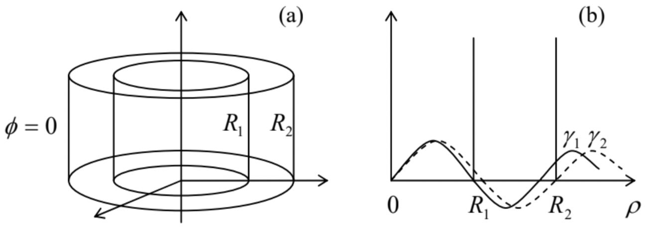Fig. 2.20. A simple boundary problem that cannot be solved using just one kind of Bessel functions.

Here two round, conducting coaxial cylindrical tubes are kept at the same (say, zero) potential, but at least one of two lids has a different potential. The problem is almost completely similar to that discussed above (Fig. 17), but now we need to find the potential distribution in the free space between the tubes, i.e. for \(\ R_{1}<\rho<R_{2}\). If we use the same variable separation as in the simpler counterpart problem, we need the radial functions \(\ \mathcal{R}(\rho)\) to satisfy two zero boundary conditions: at \(\ \rho=R_{1}\) and \(\ \rho=R_2\). With the Bessel functions of just the first kind, \(\ J_{n}(\gamma \rho)\), it is impossible to do, because the two boundaries would impose two independent (and generally incompatible) conditions, \(\ J_{n}\left(\gamma R_{1}\right)=0\), and \(\ J_{n}\left(\gamma R_{2}\right)=0\), on one “stretching parameter” \(\ \gamma\). The existence of the Bessel functions of the second kind immediately saves the day, because if the radial function solution is represented as a linear combination,

\[\ \mathcal{R}=c_{J} J_{n}(\gamma \rho)+c_{Y} Y_{n}(\gamma \rho),\tag{2.154}\]

two zero boundary conditions give two equations for \(\ \gamma\) and the ratio \(\ c \equiv c_{Y} / c_{J}\).⁴⁸ (Due to the oscillating character of both Bessel functions, these conditions would be typically satisfied by an infinite set of discrete pairs \(\ \{\gamma, c\}\).) Note, however, that generally none of these pairs would correspond to zeros of
either \(\ J_{n}\) or \(\ Y_{n}\), so that having an analog of Table 1 for the latter function would not help much. Hence, even the simplest problems of this kind (like the one shown in Fig. 20) typically require the numerical solution of transcendental algebraic equations.

In order to complete the discussion of variable separation in the cylindrical coordinates, one more issue to address is the so-called modified Bessel functions: of the first kind, \(\ I_{\nu}(\xi)\), and of the second kind, \(\ K_{\nu}(\xi)\). They are two linearly-independent solutions of the modified Bessel equation,

Modified Bessel equation

\[\ \frac{d^{2} \mathcal{R}}{d \xi^{2}}+\frac{1}{\xi} \frac{d \mathcal{R}}{d \xi}-\left(1+\frac{\nu^{2}}{\xi^{2}}\right) \mathcal{R}=0,\tag{2.155}\]

which differs from Eq. (130) “only” by the sign of one of its terms. Figure 21 shows a simple problem that leads (among many others) to this equation: a round thin conducting cylindrical pipe is sliced, perpendicular to its axis, to rings of equal height h, which are kept at equal but sign-alternating potentials.

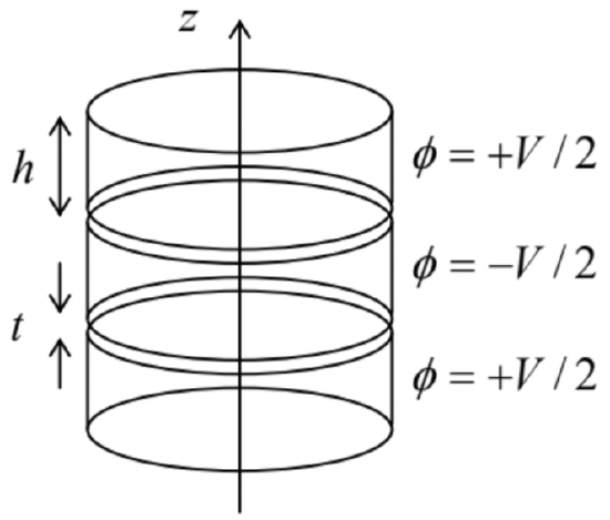Fig. 2.21. A typical boundary problem whose solution may be conveniently described in terms of the modified Bessel functions.

If the system is very long (formally, infinite) in the z-direction, we may use the variable separation method for the solution to this problem, but now we evidently need periodic (rather than exponential) solutions along the z-axis, i.e. linear combinations of \(\ \sin k z\) and \(\ \cos k z\) with various real values of the constant \(\ k\). Separating the variables, we arrive at a differential equation similar to Eq. (129), but with the negative sign before the separation constant:

\[\ \frac{d^{2} \mathcal{R}}{d \rho^{2}}+\frac{1}{\rho} \frac{d \mathcal{R}}{d \rho}-\left(k^{2}+\frac{\nu^{2}}{\rho^{2}}\right) \mathcal{R}=0.\tag{2.156}\]

The same radial coordinate’s normalization, \(\ \xi \equiv k \rho\), immediately leads us to Eq. (155), and hence (for \(\ \nu=n\)) to the modified Bessel functions \(\ I_{n}(\xi)\) and \(\ K_{n}(\xi)\).

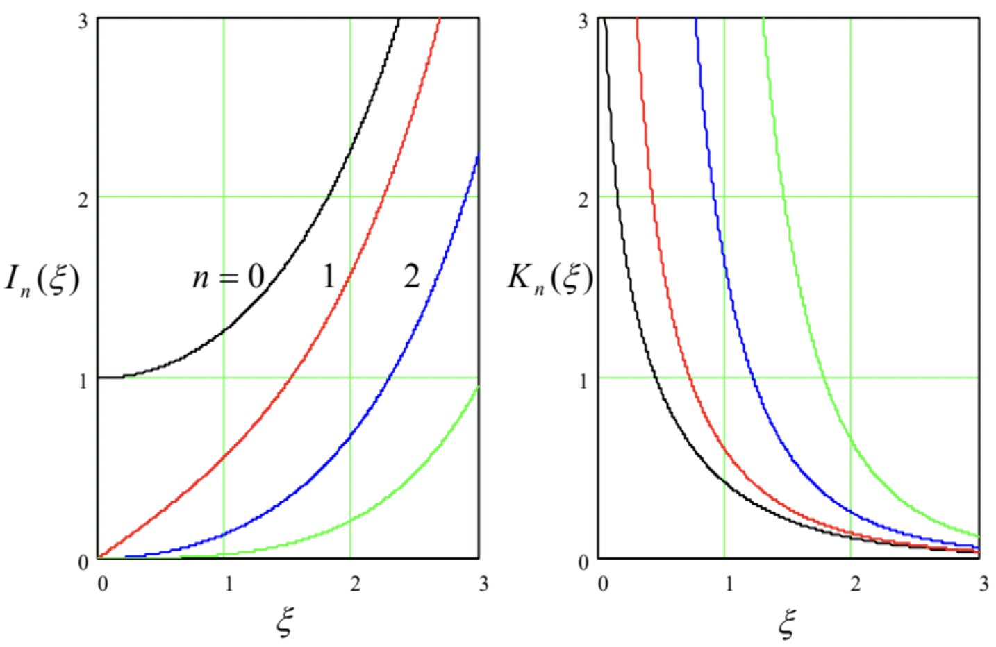
Figure 22 shows the behavior of such functions, of a few lowest orders. One can see that at \(\ \xi \rightarrow 0\) the behavior is virtually similar to that of the “usual” Bessel functions – cf. Eqs. (132) and (152), with \(\ K_{n}(\xi)\) multiplied (by purely historical reasons) by an additional coefficient, \(\ \pi / 2\):

\[\ I_{n}(\xi) \rightarrow \frac{1}{n !}\left(\frac{\xi}{2}\right)^{n}, \quad K_{n}(\xi) \rightarrow \begin{cases}-\left[\ln \left(\frac{\xi}{2}\right)+\gamma\right], & \text { for } n=0, \\ \frac{(n-1) !}{2}\left(\frac{\xi}{2}\right)^{-n}, & \text { for } n \neq 0,\end{cases}\tag{2.157}\]

However, the asymptotic behavior of the modified functions is very much different, with \(\ I_{n}(x)\) exponentially growing, and \(\ K_{n}(\xi)\) exponentially dropping at \(\ \xi \rightarrow \infty\):

\[\ I_{n}(\xi) \rightarrow\left(\frac{1}{2 \pi \xi}\right)^{1 / 2} e^{\xi}, \quad K_{n}(\xi) \rightarrow\left(\frac{\pi}{2 \xi}\right)^{1 / 2} e^{-\xi}.\tag{2.158}\]

Fig. 2.22. The modified Bessel functions of the first kind (left panel) and the second kind (right panel).

This behavior is completely natural in the context of the problem shown in Fig. 21, in which the electrostatic potential may be represented as a sum of terms proportional to \(\ I_{n}(\gamma \rho)\) inside the thin pipe, and of terms proportional to \(\ K_{n}(\gamma \rho)\) outside it.

To complete our brief survey of the Bessel functions, let me note that all of them discussed so far may be considered as particular cases of Bessel functions of the complex argument, say \(\ J_{n}(\boldsymbol{z})\) and \(\ Y_{n}(\boldsymbol{z})\), or, alternatively, \(\ H_{n}^{(1,2)}(\boldsymbol{z}) \equiv J_{n}(\boldsymbol{z}) \pm i Y_{n}(\boldsymbol{z})\).⁴⁹ At that, the “usual” Bessel functions \(\ J_{n}(\xi)\) and \(\ Y_{n}(\xi)\) may be considered as the sets of values of these generalized functions on the real axis \(\ (z=\xi)\), while the modified functions as their particular case at \(\ \boldsymbol{z}=i \xi\), also with real \(\ \xi\):

\[\ I_{\nu}(\xi)=i^{-\nu} J_{\nu}(i \xi), \quad K_{\nu}(\xi)=\frac{\pi}{2} i^{\nu+1} H_{\nu}^{(1)}(i \xi).\tag{2.159}\]

Moreover, this generalization of the Bessel functions to the whole complex plane \(\ \boldsymbol{z}\) enables the use of their values along other directions on that plane, for example under angles \(\ \pi / 4 \pm \pi / 2\). As a result, one arrives at the so-called Kelvin functions:

\[\ \begin{aligned}
&\operatorname{ber}_{\nu} \xi+i \operatorname{bei}_{\nu} \xi \equiv J_{\nu}\left(\xi e^{-i \pi / 4}\right), \\
&\operatorname{ker}_{\nu} \xi+i \operatorname{kei}_{\nu} \xi \equiv i \frac{\pi}{2} H_{\nu}^{(1)}\left(\xi e^{-i 3 \pi / 4}\right),
\end{aligned}\tag{2.160}\]

which are also useful for some important problems in physics and engineering. Unfortunately, I do not have time/space to discuss these problems in this course.⁵⁰

---

Reference

³⁹ See, e.g., MA Eq. (10.3).

⁴⁰ Note that this normalization is specific for each value of the variable separation parameter \(\ \gamma\). Also, please notice that the normalization is meaningless for \(\ \gamma=0\), i.e. for the case \(\ Z(z)=\text { const }\). However, if we need the partial solutions for this particular value of \(\ \gamma\), we can always use Eqs. (108)-(109).

⁴¹ For a more complete discussion of these functions, see the literature listed in MA Sec. 16, for example, Chapter 6 (written by F. Olver) in the famous collection compiled and edited by Abramowitz and Stegun.

⁴² These two formulas for the Bessel function peak are strictly valid for \(\ n \gg1\), but may be used for reasonable estimates starting already from \(\ n=1\); for example, \(\ \max _{\xi}\left[J_{1}(\xi)\right]\) is close to 0.58 and is reached at \(\ \xi \approx 2.4\), just about 30% away from the values given by the asymptotic formulas.

⁴³ Eq. (135) and Fig. 18 clearly show the close analogy between the Bessel functions and the usual trigonometric functions, sine and cosine. To emphasize this similarity, and help the reader to develop more gut feeling of the Bessel functions, let me mention one fact of the elasticity theory: while the sinusoidal functions describe, in particular, fundamental standing waves on a guitar string, the functions \(\ J_{n}(\xi)\) describe, in particular, fundamental standing waves on an elastic round membrane (say, a round drum), with \(\ J_{0}(\xi)\) describing their lowest (fundamental) mode – the only mode with a nonzero amplitude of the membrane center’s oscillations.

⁴⁴ Just for the reader’s reference, the Bessel functions of the same argument but different orders are also orthogonal, but differenly:

\[\ \int_{0}^{\infty} J_{n}(\xi) J_{n^{\prime}}(\xi) \frac{d \xi}{\xi}=\frac{1}{n+n^{\prime}} \delta_{n n^{\prime}}.\]

⁴⁵ These relations provide, in particular, a convenient way for numerical computation of all \(\ J_{n}(\xi)\) – after \(\ J_{0}(\xi)\) has been computed. (The latter is usually done using Eq. (132) for smaller \(\ \xi\) and an extension of Eq. (135) for larger \(\ \xi\).) Note that most mathematical software packages, including all those listed in MA Sec. 16(iv), include ready subroutines for calculation of the functions \(\ J_{n}(\xi)\) and other special functions used in this lecture series. In this sense, the line separating these “special functions” from “elementary functions” is rather fine.

⁴⁶ See, e.g., MA Eq. (6.7a). Note that \(\ \Gamma(s) \rightarrow \infty\) at \(\ s \rightarrow 0,-1,-2, \ldots\)

⁴⁷ Sometimes, they are called the Neumann functions, and denoted as \(\ N_{\nu}(\xi)\)

⁴⁸ A pair of independent linear functions, used for the representation of the general solution of the Bessel equation, may be also chosen differently, using the so-called Hankel functions

\[\ H_{n}^{(1,2)}(\xi) \equiv J_{n}(\xi) \pm i Y_{n}(\xi).\]

For representing the general solution of Eq. (130), this alternative is completely similar, for example, to using the pair of complex functions \(\ \exp \{\pm i \alpha x\} \equiv \cos \alpha x \pm i \sin \alpha x\) instead of the pair of real functions \(\ \{\cos \alpha x, \sin \alpha x\}\) for the representation of the general solution of Eq. (89) for \(\ X(x)\).

⁴⁹ These complex functions still obey the general relations (143) and (146), with \(\ \xi\) replaced with \(\ \boldsymbol{z}\).

⁵⁰ In the QM part of in this series we will run into the so-called spherical Bessel functions \(\ j_{n}(\xi)\) and \(\ y_{n}(\xi)\), which may be expressed via the Bessel functions of semi-integer orders. Surprisingly enough, these functions turn out to be simpler than \(\ J_{n}(\xi)\) and \(\ Y_{n}(\xi)\).