
4.1: Continuity Equation and the Kirchhoff Laws
- Page ID
- 56989

\( \newcommand{\vecs}[1]{\overset { \scriptstyle \rightharpoonup} {\mathbf{#1}} } \)
\( \newcommand{\vecd}[1]{\overset{-\!-\!\rightharpoonup}{\vphantom{a}\smash {#1}}} \)
\( \newcommand{\dsum}{\displaystyle\sum\limits} \)
\( \newcommand{\dint}{\displaystyle\int\limits} \)
\( \newcommand{\dlim}{\displaystyle\lim\limits} \)
\( \newcommand{\id}{\mathrm{id}}\) \( \newcommand{\Span}{\mathrm{span}}\)
( \newcommand{\kernel}{\mathrm{null}\,}\) \( \newcommand{\range}{\mathrm{range}\,}\)
\( \newcommand{\RealPart}{\mathrm{Re}}\) \( \newcommand{\ImaginaryPart}{\mathrm{Im}}\)
\( \newcommand{\Argument}{\mathrm{Arg}}\) \( \newcommand{\norm}[1]{\| #1 \|}\)
\( \newcommand{\inner}[2]{\langle #1, #2 \rangle}\)
\( \newcommand{\Span}{\mathrm{span}}\)
\( \newcommand{\id}{\mathrm{id}}\)
\( \newcommand{\Span}{\mathrm{span}}\)
\( \newcommand{\kernel}{\mathrm{null}\,}\)
\( \newcommand{\range}{\mathrm{range}\,}\)
\( \newcommand{\RealPart}{\mathrm{Re}}\)
\( \newcommand{\ImaginaryPart}{\mathrm{Im}}\)
\( \newcommand{\Argument}{\mathrm{Arg}}\)
\( \newcommand{\norm}[1]{\| #1 \|}\)
\( \newcommand{\inner}[2]{\langle #1, #2 \rangle}\)
\( \newcommand{\Span}{\mathrm{span}}\) \( \newcommand{\AA}{\unicode[.8,0]{x212B}}\)
\( \newcommand{\vectorA}[1]{\vec{#1}} % arrow\)
\( \newcommand{\vectorAt}[1]{\vec{\text{#1}}} % arrow\)
\( \newcommand{\vectorB}[1]{\overset { \scriptstyle \rightharpoonup} {\mathbf{#1}} } \)
\( \newcommand{\vectorC}[1]{\textbf{#1}} \)
\( \newcommand{\vectorD}[1]{\overrightarrow{#1}} \)
\( \newcommand{\vectorDt}[1]{\overrightarrow{\text{#1}}} \)
\( \newcommand{\vectE}[1]{\overset{-\!-\!\rightharpoonup}{\vphantom{a}\smash{\mathbf {#1}}}} \)
\( \newcommand{\vecs}[1]{\overset { \scriptstyle \rightharpoonup} {\mathbf{#1}} } \)
\(\newcommand{\longvect}{\overrightarrow}\)
\( \newcommand{\vecd}[1]{\overset{-\!-\!\rightharpoonup}{\vphantom{a}\smash {#1}}} \)
\(\newcommand{\avec}{\mathbf a}\) \(\newcommand{\bvec}{\mathbf b}\) \(\newcommand{\cvec}{\mathbf c}\) \(\newcommand{\dvec}{\mathbf d}\) \(\newcommand{\dtil}{\widetilde{\mathbf d}}\) \(\newcommand{\evec}{\mathbf e}\) \(\newcommand{\fvec}{\mathbf f}\) \(\newcommand{\nvec}{\mathbf n}\) \(\newcommand{\pvec}{\mathbf p}\) \(\newcommand{\qvec}{\mathbf q}\) \(\newcommand{\svec}{\mathbf s}\) \(\newcommand{\tvec}{\mathbf t}\) \(\newcommand{\uvec}{\mathbf u}\) \(\newcommand{\vvec}{\mathbf v}\) \(\newcommand{\wvec}{\mathbf w}\) \(\newcommand{\xvec}{\mathbf x}\) \(\newcommand{\yvec}{\mathbf y}\) \(\newcommand{\zvec}{\mathbf z}\) \(\newcommand{\rvec}{\mathbf r}\) \(\newcommand{\mvec}{\mathbf m}\) \(\newcommand{\zerovec}{\mathbf 0}\) \(\newcommand{\onevec}{\mathbf 1}\) \(\newcommand{\real}{\mathbb R}\) \(\newcommand{\twovec}[2]{\left[\begin{array}{r}#1 \\ #2 \end{array}\right]}\) \(\newcommand{\ctwovec}[2]{\left[\begin{array}{c}#1 \\ #2 \end{array}\right]}\) \(\newcommand{\threevec}[3]{\left[\begin{array}{r}#1 \\ #2 \\ #3 \end{array}\right]}\) \(\newcommand{\cthreevec}[3]{\left[\begin{array}{c}#1 \\ #2 \\ #3 \end{array}\right]}\) \(\newcommand{\fourvec}[4]{\left[\begin{array}{r}#1 \\ #2 \\ #3 \\ #4 \end{array}\right]}\) \(\newcommand{\cfourvec}[4]{\left[\begin{array}{c}#1 \\ #2 \\ #3 \\ #4 \end{array}\right]}\) \(\newcommand{\fivevec}[5]{\left[\begin{array}{r}#1 \\ #2 \\ #3 \\ #4 \\ #5 \\ \end{array}\right]}\) \(\newcommand{\cfivevec}[5]{\left[\begin{array}{c}#1 \\ #2 \\ #3 \\ #4 \\ #5 \\ \end{array}\right]}\) \(\newcommand{\mattwo}[4]{\left[\begin{array}{rr}#1 \amp #2 \\ #3 \amp #4 \\ \end{array}\right]}\) \(\newcommand{\laspan}[1]{\text{Span}\{#1\}}\) \(\newcommand{\bcal}{\cal B}\) \(\newcommand{\ccal}{\cal C}\) \(\newcommand{\scal}{\cal S}\) \(\newcommand{\wcal}{\cal W}\) \(\newcommand{\ecal}{\cal E}\) \(\newcommand{\coords}[2]{\left\{#1\right\}_{#2}}\) \(\newcommand{\gray}[1]{\color{gray}{#1}}\) \(\newcommand{\lgray}[1]{\color{lightgray}{#1}}\) \(\newcommand{\rank}{\operatorname{rank}}\) \(\newcommand{\row}{\text{Row}}\) \(\newcommand{\col}{\text{Col}}\) \(\renewcommand{\row}{\text{Row}}\) \(\newcommand{\nul}{\text{Nul}}\) \(\newcommand{\var}{\text{Var}}\) \(\newcommand{\corr}{\text{corr}}\) \(\newcommand{\len}[1]{\left|#1\right|}\) \(\newcommand{\bbar}{\overline{\bvec}}\) \(\newcommand{\bhat}{\widehat{\bvec}}\) \(\newcommand{\bperp}{\bvec^\perp}\) \(\newcommand{\xhat}{\widehat{\xvec}}\) \(\newcommand{\vhat}{\widehat{\vvec}}\) \(\newcommand{\uhat}{\widehat{\uvec}}\) \(\newcommand{\what}{\widehat{\wvec}}\) \(\newcommand{\Sighat}{\widehat{\Sigma}}\) \(\newcommand{\lt}{<}\) \(\newcommand{\gt}{>}\) \(\newcommand{\amp}{&}\) \(\definecolor{fillinmathshade}{gray}{0.9}\)Until this point, our discussion of conductors has been limited to the cases when they are separated with insulators (meaning either the free space or some dielectric media), preventing any continuous motion of charges from one conductor to another, even if there is a non-zero voltage (and hence electric field) between them – see Fig. 1a.
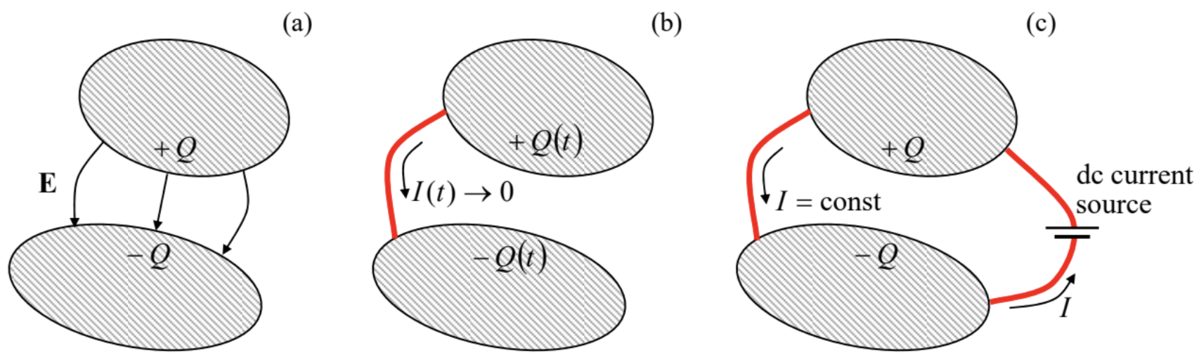
Now let us connect the two conductors with a wire – a thin, elongated conductor (Fig. 1b). Then the electric field causes the motion of charge carriers in the wire – from the conductor with a higher electrostatic potential toward that with lower potential, until the potentials equilibrate. Such a process is called charge relaxation. The main equation governing this process may be obtained from the fundamental experimental fact (already mentioned in Sec. 1.1) that electric charges cannot appear or disappear – though opposite charges may recombine with the conservation of the net charge. As a result, the charge \(\ Q\) in a conductor may change only due to the electric current \(\ I\) through the wire:
\[\ \frac{d Q}{d t}=-I(t),\tag{4.1}\]
the relation that may be understood as the definition of the current.1
Let us express Eq. (1) in a differential form, introducing the notion of the current density \(\ \mathbf{j}(\mathbf{r})\). This vector may be defined via the following relation for the elementary current \(\ dI\) crossing an elementary area \(\ dA\) (Fig. 2):
\[\ d I=j d A \cos \theta=(j \cos \theta) d A=j_{n} d A,\tag{4.2}\]
where \(\ \theta\) is the angle between the direction normal to the surface and the carrier motion direction, that is taken for the direction of the vector \(\ \mathbf{j}\).
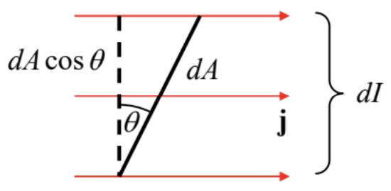 Fig. 4.2. The current density vector j.
With that definition, Eq. (1) may be rewritten as
\[\ \frac{d}{d t} \int_{V} \rho d^{3} r=-\oint_{S} j_{n} d^{2} r,\tag{4.3}\]
where \(\ V\) is an arbitrary stationary volume limited by the closed surface \(\ S\). Applying to this volume the same divergence theorem as was repeatedly used in previous chapters, we get
\[\ \int_{V}\left[\frac{\partial \rho}{\partial t}+\nabla \cdot \mathbf{j}\right] d^{3} r=0.\tag{4.4}\]
Since the volume \(\ V\) is arbitrary, this equation may be true only if
\[\ \frac{\partial \rho}{\partial t}+\nabla \cdot \mathbf{j}=0.\quad\quad\quad\quad\text{Continuity equation}\tag{4.5}\]
This is the fundamental continuity equation – which is true even for time-dependent phenomena.2
The charge relaxation, illustrated by Fig. 1b, is of course a dynamic, time-dependent process. However, electric currents may also exist in stationary situations, when a certain current source, for example a battery, drives the current against the electric field, and thus replenishes the conductor charges and sustains currents at a certain time independent level – see Fig. 1c. (This process requires a persistent replenishment of the electrostatic energy of the system from either a source or a large storage of energy of a different kind – say, the chemical energy of the battery.) Let us discuss the laws governing the distribution of such dc currents. In this case \(\ (\partial / \partial t=0)\), Eq. (5) reduces to a very simple equation
\[\ \nabla \cdot \mathbf{j}=0.\tag{4.6}\]
This relation acquires an even simpler form in the particular but important case of dc electric circuits (Fig. 3) – the systems that may be fairly represented as direct (“galvanic”) connections of components of two types:
(i) small-size (lumped) circuit elements, meaning a passive resistor, a current source, etc. – generally, any “black box” with two or more terminals, and
(ii) perfectly conducting wires, with a negligible drop of the electrostatic potential along them, that are galvanically connected at certain points called nodes (or “junctions”).
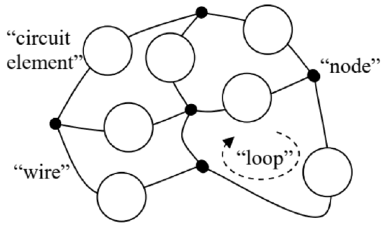 Fig. 4.3. A typical system obeying Kirchhoff laws.
In the standard circuit theory, the electric charges of the nodes are considered negligible,3 and we may integrate Eq. (6) over the closed surface drawn around any node to get a simple equality
\[\ \sum_{j} I_{j}=0,\tag{4.7a}\]
where the summation is over all the wires (numbered with index \(\ j\)) connected in the node. On the other hand, according to its definition (2.25), the voltage \(\ V_{k}\) across each circuit element may be represented as the difference of the electrostatic potentials of the adjacent nodes, \(\ V_{k}=\phi_{k}-\phi_{k-1}\). Summing such differences around any closed loop of the circuit (Fig. 3), we get all terms canceled, so that
\[\ \sum_{k} V_{k}=0.\tag{4.7b}\]
These relations are called, respectively, the \(\ 1^{s t}\) and \(\ 2^{s t}\) Kirchhoff laws4 – or sometimes the node rule (7a) and the loop rule (7b). They may seem elementary, and their genuine power is in the mathematical fact that any set of Eqs. (7), covering every node and every circuit element of the system at least once, gives a system of equations sufficient for the calculation of all currents and voltages in it – provided that the relation between the current and voltage is known for each circuit element.
It is almost evident that in the absence of current sources, the system of equations (7) has only the trivial solution: \(\ I_{j}=0, V_{k}=0\) – with the exotic exception of superconductivity, to be discussed in Sec. 6.3. The current sources, that allow non-zero current flows, may be described by their electromotive forces (e.m.f.) \(\ \mathscr{V}_{k}\), having the dimensionality of voltage, which have to be taken into account in the corresponding terms \(\ V_{k}\) of the sum (7b). Let me hope that the reader has some experience of using Eqs. (7) for analyses of simple circuits – say consisting of several resistors and batteries, so that I can save time by skipping their discussion. Still, due to their practical importance, I would recommend the reader to carry out a self-test by solving a couple of problems offered at the beginning of Sec. 6.
Reference
1 Just as a (hopefully, unnecessary :-) reminder, in the SI units the current is measured in amperes (A). In legal metrology, the ampere (rather than the coulomb, which is defined as 1C = 1A x 1s) is a primary unit. (Its formal definition will be discussed in the next chapter.) In the Gaussian units, Eq. (1) remains the same, so that the current’s unit is the statcoulomb per second – the so-called statampere.
2 Similar differential relations are valid for the density of any conserved quantity, for example for mass in the classical fluid dynamics (see, e.g., CM Sec. 8.3), and for probability in statistical physics (SM Sec. 5.6) and quantum mechanics (QM Sec. 1.4).
3 In many cases, the charge accumulation/relaxation may be described without an explicit violation of Eq. (7a), just by adding other circuit elements, lumped capacitors (see Fig. 2.5 and its discussion), to the circuit under analysis. The resulting circuit may be used to describe not only the transient processes but also periodic ac currents. However, it is convenient for me to postpone the discussion of such ac circuits until Chapter 6, where one more circuit element type, lumped inductances, will be introduced.
4 Named after Gustav Kirchhoff (1824-1887) – who also suggested the differential form (8) of the Ohm law.