7.1: Plane Waves

Let us start from considering a spatial region that does not contain field sources \(\ (\rho=0, \mathbf{j}=0)\), and is filled with a linear, uniform, isotropic medium, which obeys Eqs. (3.46) and (5.110):

\[\ \mathbf{D}=\varepsilon \mathbf{E}, \quad \mathbf{B}=\mu \mathbf{H}\tag{7.1}\]

Moreover, let us assume for a while, that these constitutive equations hold for all frequencies of interest. (Of course, these relations are exactly valid for the very important particular case of free space, where we may formally use the macroscopic Maxwell equations (6.100), but with \(\ \varepsilon=\varepsilon_{0}\) and \(\ \mu=\mu_{0}\).) As was already shown in Sec. 6.8, in this case, the Lorenz gauge condition (6.117) allows the Maxwell equations to be recast into the wave equations (6.118) for the scalar and vector potentials. However, for most purposes, it is more convenient to use the homogeneous Maxwell equations (6.100) for the electric and magnetic fields – which are independent of the gauge choice. After an elementary elimination of \(\ \mathbf{D}\) and \(\ \mathbf{B}\) using Eqs. (1),¹ these equations take a simple, very symmetric form:

\(\ \text{Maxwell equations for uniform linear media}\quad\quad\quad\quad\begin{array}{llr}
\nabla \times \mathbf{E}+\mu \frac{\partial \mathbf{H}}{\partial t}=0, & \nabla \times \mathbf{H}-\varepsilon \frac{\partial \mathbf{E}}{\partial t}=0, \quad\quad\quad&(7.2a)\\
\nabla \cdot \mathbf{E}=0, & \nabla \cdot \mathbf{H}=0.&(7.2b)
\end{array}\)

Now, acting by operator \(\ \nabla \times\) on each of Eqs. (2a), i.e. taking their curl, and then using the vector algebra identity (5.31), whose first term, for both \(\ \mathbf{E}\) and \(\ \mathbf{H}\), vanishes due to Eqs. (2b), we get fully similar wave equations for the electric and magnetic fields:²

\[\ \text{EM wave equations}\quad\quad\quad\quad\left(\nabla^{2}-\frac{1}{\nu^{2}} \frac{\partial^{2}}{\partial t^{2}}\right) \mathbf{E}=0, \quad\left(\nabla^{2}-\frac{1}{\nu^{2}} \frac{\partial^{2}}{\partial t^{2}}\right) \mathbf{H}=0,\tag{7.3}\]

where the parameter v is defined as

\[\ \nu^{2} \equiv \frac{1}{\varepsilon \mu}.\quad\quad\quad\quad\text{Wave velocity}\tag{7.4}\]

with \(\ \nu^{2}=1 / \varepsilon_{0} \mu_{0} \equiv c^{2}\) in free space – see Eq. (6.120) again.

These equations allow, in particular, solutions of the following particular type;

\[\ E \propto H \propto f(z-\nu t),\quad\quad\quad\quad\text{Plane wave}\tag{7.5}\]

where \(\ z\) is the Cartesian coordinate along a certain (arbitrary) direction n, and f is an arbitrary function of one argument. This solution describes a specific type of a traveling wave – meaning a certain field pattern moving, without deformation, along the z-axis, with velocity v. According to Eq. (5), both E and H have the same values at all points of each plane perpendicular to the direction \(\ \mathbf{n} \equiv \mathbf{n}_{z}\) of the wave propagation; hence the name – plane wave.

According to Eqs. (2), the independence of the wave equations (3) for vectors E and H does not mean that their plane-wave solutions are independent. Indeed, plugging any solution of the type (5) into Eqs. (2a), we get

\[\ \mathbf{H}=\frac{\mathbf{n} \times \mathbf{E}}{Z}, \quad \text { i.e. } \mathbf{E}=Z \mathbf{H} \times \mathbf{n},\quad\quad\quad\quad\text{Field vector relationship}\tag{7.6}\]

where

\[\ Z \equiv \frac{E}{H}=\left(\frac{\mu}{\varepsilon}\right)^{1 / 2}.\quad\quad\quad\quad\text{Wave
impedance}\tag{7.7}\]

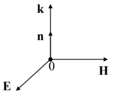
The vector relationship (6) means, first of all, that the vectors E and H are perpendicular not only to the propagation vector n (such waves are called transverse), but also to each other (Fig. 1) – at any point of space and at any time instant. Second, this equality does not depend on the function \(\ f\), meaning that the electric and magnetic fields increase and decrease simultaneously.

Fig. 7.1. Field vectors in a plane electromagnetic n.

Finally, the field magnitudes are related by the constant \(\ Z\), called the wave impedance of the medium. Very soon we will see that the impedance plays a pivotal role in many problems, in particular at the wave reflection from the interface between two media. Since the dimensionality of \(\ E\), in SI units, is V/m, and that of \(\ H\) is A/m, Eq. (7) shows that \(\ Z\) has the dimensionality of V/A, i.e. ohms \(\ (\Omega)\).³ In particular, in free space,

\[\ \text{Wave impedance of free space}\quad\quad\quad\quad Z=Z_{0} \equiv\left(\frac{\mu_{0}}{\varepsilon_{0}}\right)^{1 / 2}=4 \pi \times 10^{-7} c \approx 377 \Omega.\tag{7.8}\]

Next, plugging Eq. (6) into Eqs. (6.113) and (6.114), we get:

\[\ \text{Wave’s energy}\quad\quad\quad\quad u=\varepsilon E^{2}=\mu H^{2},\tag{7.9a}\]

\[\ \text{Wave’s power}\quad\quad\quad\quad \mathbf{S} \equiv \mathbf{E} \times \mathbf{H}=\mathbf{n} \frac{E^{2}}{Z}=\mathbf{n} Z H^{2},\tag{7.9b}\]

so that, according to Eqs. (4) and (7), the wave’s energy and power densities are universally related as

\[\ \mathbf{S}=\mathbf{n} u \nu.\tag{7.9c}\]

In the view of the Poynting vector paradox discussed in Sec. 6.8 (see Fig. 6.11), one may wonder whether the last equality may be interpreted as the actual density of power flow. In contrast to the static situation shown in Fig. 6.11, which limits the electric and magnetic fields to vicinity of their sources, waves may travel far from them. As a result, they can form wave packets of a finite length in free space – see Fig. 2.

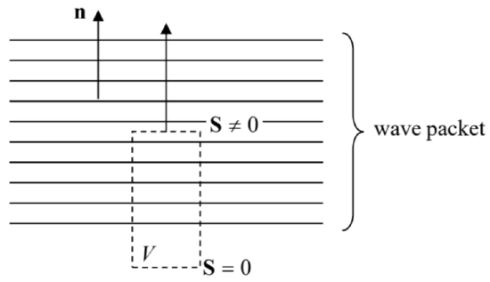Fig. 7.2. Interpreting the Poynting vector in a plane electromagnetic wave. (Horizontal lines show equal-field planes.)

Let us apply the Poynting theorem (6.111) to the cylinder shown with dashed lines in Fig. 2, with one lid inside the wave packet, and another lid in the region already passed by the wave. Then, according to Eq. (6.111), the rate of change of the full field energy \(\ \mathscr{E}\) inside the volume is \(\ d \mathscr{E} / d t=-S A\) (where \(\ A\) is the lid area), so that \(\ S\) may be indeed interpreted as the power flow (per unit area) from the volume. Making a reasonable assumption that the finite length of a sufficiently long wave packet does not affect the physics inside it, we may indeed interpret the \(\ \mathbf{S}\) given by Eqs. (9b-c) as the power flow
density inside a plane electromagnetic wave.

As we will see later in this chapter, the free-space value \(\ Z_{0}\) of the wave impedance, given by Eq. (8), establishes the scale of \(\ Z\) of virtually all wave transmission lines, so we may use it, together with Eq. (9), to get a better feeling of how much different are the electric and magnetic field amplitudes in the waves – on the scale of typical electrostatics and magnetostatics experiments. For example, according to Eqs. (9), a wave of a modest intensity \(\ S=1 \mathrm{~W} / \mathrm{m}^{2}\) (this is what we get from a usual electric bulb a few meters away from it) has \(\ E \sim\left(S Z_{0}\right)^{1 / 2} \sim 20 \mathrm{~V} / \mathrm{m}\), quite comparable with the dc field created by a standard AA battery right outside it. On the other hand, the wave’s magnetic field \(\ H=\left(S / Z_{0}\right)^{1 / 2} \approx 0.05 \mathrm{~A} / \mathrm{m}\). For this particular case, the relation following from Eqs. (1), (4), and (7),

\[\ B=\mu H=\mu \frac{E}{Z}=\mu \frac{E}{(\mu / \varepsilon)^{1 / 2}} \equiv(\varepsilon \mu)^{1 / 2} E=\frac{E}{\nu},\tag{7.10}\]

gives \(\ B=\mu_{0} H=E / c \sim 7 \times 10^{-8} \mathrm{~T}\), i.e. a magnetic field a thousand times lower than the Earth’s field, and about 7 orders of magnitude lower than the field of a typical permanent magnet. This huge difference may be interpreted as follows: the scale of magnetic fields \(\ B \sim E / c\) in the waves is “normal” for electromagnetism, while the permanent magnet fields are abnormally high because they are due to the ferromagnetic alignment of electron spins, essentially relativistic objects – see the discussion in Sec. 5.5.

The fact that Eq. (5) is valid for an arbitrary function \(\ f\) means, in plain English, that a medium with frequency-independent \(\ \varepsilon\) and \(\ \mu\) supports propagation of plane waves with an arbitrary waveform – without either decay (attenuation) or deformation (dispersion). However, for any real medium but vacuum, this approximation is valid only within limited frequency intervals. We will discuss the effects of attenuation and dispersion in the next section and will see that all our prior formulas remain valid even for an arbitrary linear media, provided that we limit them to single-frequency (i.e. sinusoidal, frequently called monochromatic) waves. Such waves may be most conveniently represented as⁴

where \(\ f_{\omega}\) is the complex amplitude of the wave, and \(\ k\) is its wave number (the magnitude of the wave vector \(\ \mathbf{k} \equiv \mathbf{n} k\)), sometimes also called the spatial frequency. The last term is justified by the fact, evident from Eq. (11), that \(\ k\) is related to the wavelength \(\ \lambda\) exactly as the usual (“temporal”) frequency \(\ \omega\) is related to the time period \(\ \tau\):

\[\ k=\frac{2 \pi}{\lambda}, \quad \omega=\frac{2 \pi}{\tau}.\quad\quad\quad\quad\text{Spatial and temporal frequencies}\tag{7.12}\]

In the “dispersion-free” case (5), the compatibility of that relation with Eq. (11) requires the argument \(\ (k z-\omega t) \equiv k[z-(\omega / k) t]\) to be proportional to \(\ (z-\nu t)\), so that \(\ \omega / k=\nu\), i.e.

\[\ k=\frac{\omega}{\nu} \equiv(\varepsilon \mu)^{1 / 2} \omega,\quad\quad\quad\quad\text{Dispersion
relation}\tag{7.13}\]

so that in that particular case, the dispersion relation \(\ \omega(k)\) is linear.

Now note that Eq. (6) does not mean that the vectors E and H retain their direction in space. (The wave in that they do is called linearly-polarized.⁵) Indeed, nothing in the Maxwell equations prevents, for example, a joint rotation of this pair of vectors around the fixed vector n, while still keeping all these three vectors perpendicular to each other at any instant – see Fig. 1. However, an arbitrary rotation law or even an arbitrary constant frequency of such rotation would violate the single- frequency (monochromatic) character of the elementary sinusoidal wave (11). To understand what is the most general type of polarization the wave may have without violating that condition, let us represent two Cartesian components of one of these vectors (say, E) along any two fixed axes \(\ x\) and \(\ y\), perpendicular to each other and the z-axis (i.e. to the vector n), in the same form as used in Eq. (11):

\[\ E_{x}=\operatorname{Re}\left[E_{\omega x} e^{i(k z-\omega t)}\right], \quad E_{y}=\operatorname{Re}\left[E_{\omega y} e^{i(k z-\omega t)}\right].\tag{7.14}\]

To keep the wave monochromatic, the complex amplitudes \(\ E_{\omega x}\) and \(\ E_{\omega y}\) have to be constant in time; however, they may have different magnitudes and an arbitrary phase shift between them.

In the simplest case when the arguments of these complex amplitudes are equal,

\[\ E_{\omega x, y}=\left|E_{\omega x, y}\right| e^{i \varphi}.\tag{7.15}\]

the real field components have the same phase:

\[\ E_{x}=\left|E_{\omega x}\right| \cos (k z-\omega t+\varphi), \quad E_{y}=\left|E_{\omega y}\right| \cos (k z-\omega t+\varphi),\tag{7.16}\]

so that their ratio is constant in time – see Fig. 3a. This means that the wave is linearly polarized, with the polarization plane defined by the relation

\[\ \tan \theta=\left|E_{\omega y}\right| /\left|E_{\omega x}\right|.\tag{7.17}\]

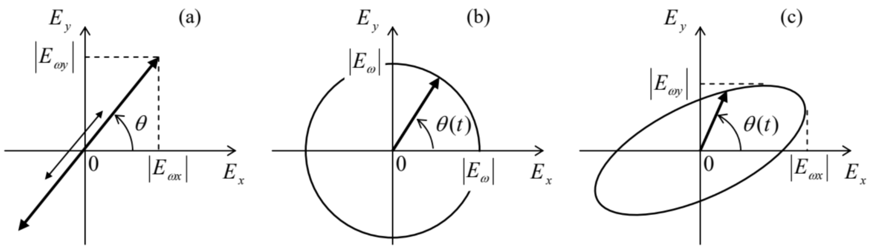Fig. 7.3. Time evolution of the instantaneous electric field vector in monochromatic waves with: (a) a linear polarization, (b) a circular polarization, and (c) an elliptical polarization.

Another simple case is when the moduli of the complex amplitudes \(\ E_{\omega x}\) and \(\ E_{\omega y}\) are equal, but their phases are shifted by \(\ +\pi / 2\) or \(\ -\pi / 2\):

\[\ E_{\omega x}=\left|E_{\omega}\right| e^{i \varphi}, \quad E_{\omega y}=\left|E_{\omega}\right| e^{i(\varphi \pm \pi / 2)}.\tag{7.18}\]

In this case

\[\ E_{x}=\left|E_{\omega}\right| \cos (k z-\omega t+\varphi), \quad E_{y}=\left|E_{\omega}\right| \cos \left(k z-\omega t+\varphi \pm \frac{\pi}{2}\right) \equiv \mp\left|E_{\omega}\right| \sin (k z-\omega t+\varphi).\tag{7.19}\]

This means that on the wave’s plane (normal to n), the end of the vector E moves, with the wave’s frequency \(\ \omega\), either clockwise or counterclockwise around a circle – see Fig. 3b:

\[\ \theta(t)=\mp(\omega t-\varphi).\tag{7.20}\]

Such waves are called circularly-polarized. In the dominant convention, the wave is called right-polarized (RP) if it is described by the lower sign in Eqs. (18)-(20), i.e. if the vector \(\ \mathbf{\omega}\) of the angular frequency of the field vector’s rotation coincides with the wave propagation’s direction n, and left-polarized (LP) in the opposite case. These particular solutions of the Maxwell equations are very convenient for quantum electrodynamics, because single electromagnetic field quanta with a certain (positive or negative) spin direction may be considered as elementary excitations of the corresponding circularly-polarized wave.⁶ (This fact does not exclude, from the quantization scheme, waves of other polarizations, because any monochromatic wave may be presented as a linear combination of two opposite circularly-polarized waves – just as Eqs. (14) represent it as a linear combination of two linearly-polarized waves.)

Finally, in the general case of arbitrary complex amplitudes \(\ E_{\omega x}\) and \(\ E_{\omega y}\), the field vector’s end moves along an ellipse (Fig. 3c); such wave is called elliptically polarized. The elongation (“eccentricity”) and orientation of the ellipse are completely described by one complex number, the ratio \(\ E_{\omega x} / E_{\omega y}\), i.e. by two real numbers, for example, \(\ \left|E_{\omega x} / E_{\omega y}\right|\) and \(\ \varphi=\arg \left(E_{\omega x} / E_{\omega y}\right)\).⁷

---

Reference

¹ Though B rather than H is the actual magnetic field, mathematically it is a bit more convenient (just as it was in Sec. 6.2) to use the vector pair \(\ \{\mathbf{E}, \mathbf{H}\}\) in the following discussion, because at sharp media boundaries, it is H that obeys the boundary condition (5.117) similar to that for E – cf. Eq. (3.37).

² The two vector equations (3) are of course is just a shorthand for six similar equations for three Cartesian components of E and H, and hence for their magnitudes \(\ E\) and \(\ H\).

³ In the Gaussian units, \(\ E\) and \(\ H\) have a similar dimensionality (in particular, in a free-space wave, \(\ E = H\)), making the (very useful) notion of the wave impedance less manifestly exposed – so that in some older physics textbooks it is not mentioned at all!

⁴ As we have already seen in the previous chapter (see also CM Sec. 1), such complex-exponential representation of sinusoidally-changing variables is more convenient for mathematical manipulation with that using sine and cosine functions, especially because in all linear relations, the operator Re may be omitted (implied) until the very end of the calculation. Note, however, that this is not valid for the quadratic forms such as Eqs. (9a-b).

⁵ The possibility of different polarizations of electromagnetic waves was discovered (for light) in 1699 by Rasmus Bartholin, a.k.a. Erasmus Bartholinus.

⁶ This issue is closely related to that of the wave’s angular momentum; it will be more convenient for me to discuss it later in this chapter (in Sec. 7).

⁷ Note that the same information may be expressed via four so-called Stokes parameters \(\ s_{0}, s_{1}, s_{2}, s_{3}\), which are popular in practical optics, because they may be used for the description of not only completely coherent waves that are discussed here, but also of party coherent or even fully incoherent waves – including the natural light emitted by thermal sources such as our Sun. (In contrast to the coherent waves (14), whose complex amplitudes are deterministic numbers, the amplitudes of incoherent waves should be treated as random variables.) For more on the Stokes parameters, as well as many other optics topics I will not have time to cover, I can recommend the classical text by M. Born et al., Principles of Optics, 7th ed., Cambridge U. Press, 1999.