7.2: Attenuation and Dispersion

Let me start the discussion of the dispersion and attenuation effects by considering a particular case of time evolution of the electric polarization \(\ \mathbf{P}(t)\) of a dilute, non-polar medium, with negligible interaction between its elementary dipoles \(\ \mathbf{p}(t)\). As was discussed in Sec. 3.3, in this case, the local electric field acting on each elementary dipole, is equal to the macroscopic field \(\ \mathbf{E}(t)\). Then, the dipole moment \(\ \mathbf{p}(t)\) may be caused not only by the values of the field E at the same moment of time \(\ (t)\), but also those at the earlier moments, \(\ t<t’\). Due to the linear superposition principle, the macroscopic polarization \(\ \mathbf{P}(t)=n \mathbf{p}(t)\) should be a sum (or rather an integral) of the values of \(\ \mathbf{E}\left(t^{\prime}\right)\) at all moments \(\ t^{\prime} \leq t\), weighed by some function of \(\ t\) and \(\ t’\):⁸

\[\ P(t)=\int_{-\infty}^{t} E\left(t^{\prime}\right) G\left(t, t^{\prime}\right) d t^{\prime}.\quad\quad\quad\quad\text{Temporal Green’s function}\tag{7.21}\]

The condition \(\ t^{\prime} \leq t\), which is implied by this relation, expresses a keystone principle of physics, the causal relation between a cause (in our case, the electric field applied to each dipole) and its effect (the polarization it creates). The function \(\ G\left(t, t^{\prime}\right)\) is called the temporal Green’s function for the electric
polarization.⁹ To reveal its physical sense, let us consider the case when the applied field \(\ E(t)\) is a very short pulse at the moment \(\ t_{0}<t\), which may be well approximated with the Dirac’s delta function:

\[\ E(t)=\delta\left(t-t^{\prime \prime}\right).\tag{7.22}\]

Then Eq. (21) yields just \(\ P(t)=G\left(t, t^{\prime \prime}\right)\), so that the Green’s function \(\ G\left(t, t^{\prime}\right)\) is just the polarization at moment \(\ t\), created by a unit \(\ \delta \text {-functional }\) pulse of the applied field at moment \(\ t^{\prime}\) (Fig. 4).

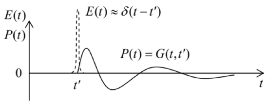Fig. 7.4. An example of the temporal Green’s function for the electric polarization (schematically).

What are the general properties of the temporal Green’s function? First, the function is real, since the dipole moment \(\ \mathbf{p}\) and hence the polarization \(\ \mathbf{P}=n \mathbf{p}\) are real – see Eq. (3.6). Next, for systems without infinite internal “memory”, \(\ G\) should tend to zero at \(\ t-t^{\prime} \rightarrow \infty\), although the type of this approach (e.g., whether the function G oscillates approaching zero, as in Fig. 4, or not) depends on the medium’s properties. Finally, if parameters of the medium do not change in time, the polarization response to an electric field pulse should be dependent not on its absolute timing, but only on the time difference \(\ \theta \equiv t-t^{\prime}\) between the pulse and observation instants, i.e. Eq. (21) is reduced to

\[\ P(t)=\int_{-\infty}^{t} E\left(t^{\prime}\right) G\left(t-t^{\prime}\right) d t^{\prime} \equiv \int_{0}^{\infty} E(t-\theta) G(\theta) d \theta.\tag{7.23}\]

For a sinusoidal waveform, \(\ E(t)=\operatorname{Re}\left[E_{\omega} e^{-i \omega t}\right]\), this equation yields

\[\ P(t)=\operatorname{Re} \int_{0}^{\infty} E_{\omega} e^{-i \omega(t-\theta)} G(\theta) d \theta \equiv \operatorname{Re}\left[\left(E_{\omega} \int_{0}^{\infty} G(\theta) e^{i \omega \theta} d \theta\right) e^{-i \omega t}\right].\tag{7.24}\]

The expression in the last parentheses is of course nothing else than the complex amplitude \(\ P_{\omega}\) of the polarization. This means that though even if the static linear relation (3.43), \(\ P=\chi_{\mathrm{e}} \varepsilon_{0} E\), is invalid for an arbitrary time-dependent process, we may still keep its Fourier analog,

\[\ P_{\omega}=\chi_{\mathrm{e}}(\omega) \varepsilon_{0} E_{\omega}, \quad \text { with } \chi_{\mathrm{e}}(\omega) \equiv \frac{1}{\varepsilon_{0}} \int_{0}^{\infty} G(\theta) e^{i \omega \theta} d \theta,\tag{7.25}\]

for each sinusoidal component of the process, using it as the definition of the frequency-dependent electric susceptibility \(\ \chi_{\mathrm{e}}(\omega)\). Similarly, the frequency-dependent electric permittivity may be defined using the Fourier analog of Eq. (3.46):

\[\ D_{\omega} \equiv \varepsilon(\omega) E_{\omega}.\quad\quad\quad\quad \text{Complex electric permittivity}\tag{7.26a}\]

Then, according to the definition (3.33), the permittivity is related to the temporal Green’s function by the usual Fourier transform:

\[\ \varepsilon(\omega) \equiv \varepsilon_{0}+\frac{P_{\omega}}{E_{\omega}}=\varepsilon_{0}+\int_{0}^{\infty} G(\theta) e^{i \omega \theta} d \theta.\tag{7.26b}\]

This relation shows that \(\ \varepsilon(\omega)\) may be complex,

\[\ \varepsilon(\omega)=\varepsilon^{\prime}(\omega)+i \varepsilon^{\prime \prime}(\omega), \quad \text { with } \varepsilon^{\prime}(\omega)=\varepsilon_{0}+\int_{0}^{\infty} G(\theta) \cos \omega \theta d \theta, \quad \varepsilon^{\prime \prime}(\omega)=\int_{0}^{\infty} G(\theta) \sin \omega \theta d \theta,\tag{7.27}\]

and that its real part \(\ \varepsilon^{\prime}(\omega)\) is always an even function of frequency, while the imaginary part \(\ \varepsilon^{\prime \prime}(\omega)\) is an
odd function of \(\ \omega\). Note that though the particular causal relationship (21) between \(\ P(t)\) and \(\ E(t)\) is conditioned by the elementary dipole independence, the frequency-dependent complex electric permittivity \(\ \varepsilon(\omega)\) may be introduced, in a similar way, if any two linear combinations of these variables are related by a similar formula. Absolutely similar arguments show that magnetic properties of a linear, isotropic medium may be characterized with a frequency-dependent, complex permeability \(\ \mu(\omega)\).

Now rewriting Eqs. (1) for the complex amplitudes of the fields at a particular frequency, we may repeat all calculations of Sec. 1, and verify that all its results are valid for monochromatic waves even for a dispersive (but necessarily linear!) medium. In particular, Eqs. (7) and (13) now become

\[\ Z(\omega)=\left(\frac{\mu(\omega)}{\varepsilon(\omega)}\right)^{1 / 2}, \quad k(\omega)=\omega[\varepsilon(\omega) \mu(\omega)]^{1 / 2},\quad\quad\quad\quad\text{Complex } Z \text{ and } k\tag{7.28}\]

so that the wave impedance and the wave number may be both complex functions of frequency.¹⁰

This fact has important consequences for electromagnetic wave propagation. First, plugging the representation of the complex wave number as the sum of its real and imaginary parts, \(\ k(\omega) \equiv k^{\prime}(\omega)+ik^{\prime\prime}(\omega)\), into Eq. (11):

\[\ f=\operatorname{Re}\left\{f_{\omega} e^{i[k(\omega) z-\omega t]}\right\}=e^{-k^{\prime \prime}(\omega) z} \operatorname{Re}\left\{f_{\omega} e^{i\left[k^{\prime}(\omega) z-\omega t\right]}\right\},\tag{7.29}\]

we see that \(\ k^{\prime \prime}(\omega)\) describes the rate of wave attenuation in the medium at frequency \(\ \omega\).¹¹ Second, if the waveform is not sinusoidal (and hence should be represented as a sum of several/many sinusoidal components), the frequency dependence of \(\ k^{\prime}(\omega)\) provides for wave dispersion, i.e. the waveform deformation at the propagation, because the propagation velocity (4) of component waves is now different.¹²

As an example of such a dispersive medium, let us consider a simple but very representative Lorentz oscillator model.¹³ In dilute atomic or molecular systems (e.g., gases), electrons respond to the external electric field especially strongly when frequency \(\ \omega\) is close to certain frequencies \(\ \omega_{j}\) corresponding to the spectrum of quantum interstate transitions of a single atom/molecule. An approximate, phenomenological description of this behavior may be obtained from a classical model of several externally-driven harmonic oscillators, generally with non-zero damping. For a single oscillator, driven by the electric field’s force \(\ F(t)=q E(t)\), we can write the \(\ 2^{\text {nd }}\) Newton law as

\[\ m\left(\ddot{x}+2 \delta_{0} \dot{x}+\omega_{0}^{2} x\right)=q E(t),\tag{7.30}\]

where \(\ \omega_{0}\) is the own frequency of the oscillator, and \(\ \delta_{0}\) its damping coefficient. For the electric field of a monochromatic wave, \(\ E(t)=\operatorname{Re}\left[E_{\omega} \exp \{-i \omega t\}\right]\), we may look for a particular, forced-oscillation solution of this equation in a similar form \(\ x(t)=\operatorname{Re}\left[x_{\omega} \exp \{-i \omega t\}\right]\).¹⁴ Plugging this solution into Eq. (30), we readily find the complex amplitude of these oscillations:

\[\ x_{\omega}=\frac{q}{m} \frac{E_{\omega}}{\left(\omega_{0}^{2}-\omega^{2}\right)-2 i \omega \delta_{0}}.\tag{7.31}\]

Using this result to calculate the complex amplitude of the dipole moment as \(\ p_{\omega}=q x_{\omega}\), and then the electric polarization \(\ P_{\omega}=n p_{\omega}\) of a dilute medium with \(\ n\) independent oscillators for unit volume, for its frequency-dependent permittivity (26) we get

\[\ \text{Lorentz oscillator model}\quad\quad\quad\quad\varepsilon(\omega)=\varepsilon_{0}+n \frac{q^{2}}{m} \frac{1}{\left(\omega_{0}^{2}-\omega^{2}\right)-2 i \omega \delta_{0}}.\tag{7.32}\]

This result may be readily generalized to the case when the system has several types of oscillators with different masses and frequencies:

\[\ \varepsilon(\omega)=\varepsilon_{0}+n q^{2} \sum_{j} \frac{f_{j}}{m_{j}\left[\left(\omega_{j}^{2}-\omega^{2}\right)-2 i \omega \delta_{j}\right]},\tag{7.33}\]

where \(\ f_{j} \equiv n_{j} / n\) is the fraction of oscillators with frequency \(\ \omega_{j}\), so that the sum of all \(\ f_{j}\) equals 1. Figure 5 shows a typical behavior of the real and imaginary parts of the complex dielectric constant, described by Eq. (33), as functions of frequency. The oscillator resonances’ effect is clearly visible, and dominates the media response at \(\ \omega \approx \omega_{j}\), especially in the case of low damping, \(\ \delta_{j}<<\omega_{j}\). Note that in the low-damping limit, the imaginary part of the dielectric constant \(\ \varepsilon^{\prime \prime}\), and hence the wave attenuation \(\ k^{\prime \prime}\), are negligibly small at all frequencies besides small vicinities of frequencies \(\ \omega_{j}\), where the derivative \(\ d \varepsilon^{\prime}(\omega) / d \omega\) is negative.¹⁵ Thus, for a system of for weakly-damped oscillators, Eq. (33) may be well approximated by a sum of singularities (“poles”):

\[\ \varepsilon(\omega) \approx \varepsilon_{0}+n \frac{q^{2}}{2} \sum_{j} \frac{f_{j}}{m_{j} \omega_{j}\left(\omega_{j}-\omega\right)}, \quad \text { for } \delta_{j}<<\left|\omega-\omega_{j}\right|<<\left|\omega_{j}-\omega_{j^{\prime}}\right|.\tag{7.34}\]

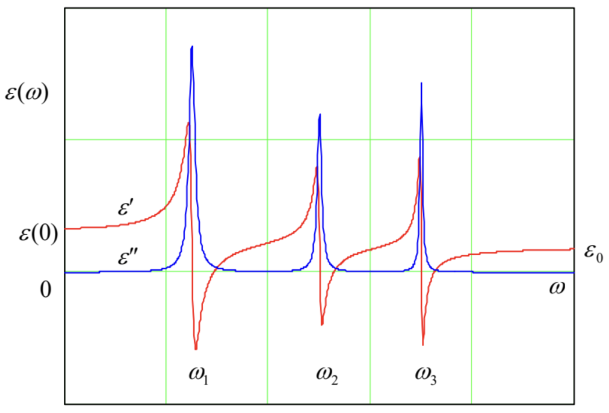Fig. 7.5. Typical frequency dependence of the real and imaginary parts of the complex electric permittivity, according to the generalized Lorentz oscillator model.

This result is especially important because, according to quantum mechanics,¹⁶ Eq. (34) (with all \(\ m_{j}\) equal) is also valid for a set of non-interacting, similar quantum systems (whose dynamics may be completely different from that of a harmonic oscillator!), provided that \(\ \omega_{j}\) are replaced with frequencies
of possible quantum interstate transitions, and coefficients \(\ f_{j}\) are replaced with the so-called oscillator strengths of the transitions – which obey the same sum rule, \(\ \sum_{j} f_{j}=1\).

At \(\ \omega \rightarrow 0\), the imaginary part of the permittivity (33) also vanishes (for any \(\ \delta_{j}\)), while its real part approaches its electrostatic (“dc”) value

\[\ \varepsilon(0)=\varepsilon_{0}+q^{2} \sum_{j} \frac{n_{j}}{m_{j} \omega_{j}^{2}}.\tag{7.35}\]

Note that according to Eq. (30), the denominator in Eq. (35) is just the effective spring constant \(\ \kappa_{j}=m_j\omega_j^2\) of the \(\ j^{\text {th }}\) oscillator, so that the oscillator masses \(\ m_{j}\) as such are actually (and quite naturally) not involved in the static dielectric response.

In the opposite limit of very high frequencies, \(\ \omega >> \omega_{j}, \delta_{j}\), the permittivity also becomes real and may be represented as

\[\ \varepsilon(\omega)=\varepsilon_{0}\left(1-\frac{\omega_{\mathrm{p}}^{2}}{\omega^{2}}\right), \quad \text { where } \omega_{\mathrm{p}}^{2} \equiv \frac{q^{2}}{\varepsilon_{0}} \sum_{j} \frac{n_{j}}{m_{j}}\quad\quad\quad\quad \varepsilon(\omega) \text{ in plasma} \tag{7.36}\]

This result is very important, because it is also valid at all frequencies if all \(\ \omega_{j}\) and \(\ \delta_{j}\) vanish, for example for gases of free charged particles, in particular for plasmas – ionized atomic gases, provided that the ion collision effects are negligible. (This is why the parameter \(\ \omega_{\mathrm{p}}\) defined by Eq. (36) is called the plasma frequency.) Typically, the plasma as a whole is neutral, i.e. the density \(\ n\) of positive atomic ions is equal to that of the free electrons. Since the ratio \(\ n_{j} / m_{j}\) for electrons is much higher than that for ions, the general formula (36) for the plasma frequency is usually well approximated by the following simple expression:

\[\ \omega_{\mathrm{p}}^{2}=\frac{n e^{2}}{\varepsilon_{0} m_{\mathrm{e}}}.\tag{7.37}\]

This expression has a simple physical sense: the effective spring constant \(\ \kappa_{\mathrm{ef}} \equiv m_{\mathrm{e}} \omega_{\mathrm{p}}^{2}=n e^{2} / \varepsilon_{0}\) describes the Coulomb force that appears when the electron subsystem of the plasma is shifted, as a whole, from its positive-ion subsystem, thus violating the electroneutrality. (Indeed, let us consider such a small shift, \(\ \Delta x\), perpendicular to the plane surface of a broad, plane slab filled with plasma. The uncompensated ion charges, with equal and opposite surface densities \(\ \sigma=\pm e n \Delta x\), that appear at the slab surfaces, create inside it, according to Eq. (2.3), a uniform electric field with \(\ E_{x}=e n \Delta x / \varepsilon_{0}\). This field exerts force \(\ -e E=-\left(n e^{2} / \varepsilon_{0}\right) \Delta x=-\kappa_{\mathrm{ef}} \Delta x\) on each electron, pulling it back to its equilibrium position.) Hence, there is no surprise that the function \(\ \varepsilon(\omega)\) given by Eq. (36) vanishes at \(\ \omega=\omega_{\mathrm{p}}\): at this resonance frequency, the polarization electric field E may oscillate, i.e. have a non-zero amplitude \(\ E_{\omega}=D_{\omega} / \varepsilon(\omega)\), even in the absence of external forces induced by external (stand-alone) charges, i.e. in the absence of the field D these charges induce – see Eq. (3.32).

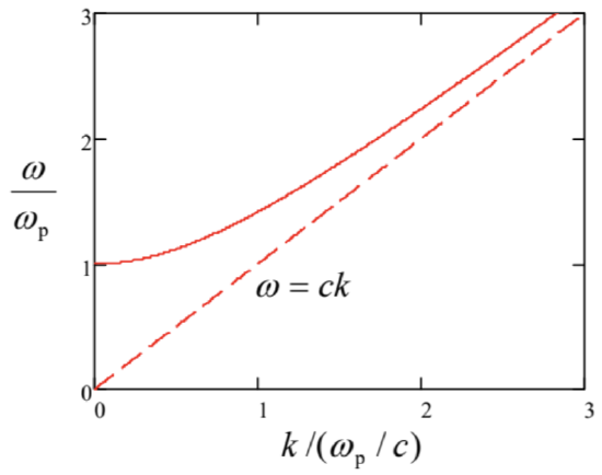
The behavior of electromagnetic waves in a medium that obeys Eq. (36), is very remarkable. If the wave frequency \(\ \omega\) is above \(\ \omega_{\mathrm{p}}\), the dielectric constant \(\ \varepsilon(\omega)\), and hence the wave number (28) are positive and real, and waves propagate without attenuation, following the dispersion relation,

\[\ \text{Plasma dispersion relation}\quad \quad\quad\quad k(\omega)=\omega\left[\varepsilon(\omega) \mu_{0}\right]^{1 / 2}=\frac{1}{c}\left(\omega^{2}-\omega_{\mathrm{p}}^{2}\right)^{1 / 2},\tag{7.38}\]

which is shown in Fig. 6.

Fig. 7.6. The plasma dispersion law (solid line) in comparison with the linear dispersion in the free space (dashed line).

At \(\ \omega \rightarrow \omega_{\mathrm{p}}\) the wave number \(\ k\) tends to zero. Beyond that point (i.e. at \(\ \omega<\omega_{\mathrm{p}}\)), we still can use
Eq. (38), but it is instrumental to rewrite it in the mathematically equivalent form

\[\ k(\omega)=\frac{i}{c}\left(\omega_{\mathrm{p}}^{2}-\omega^{2}\right)^{1 / 2}=\frac{i}{\delta}, \quad \text { where } \delta \equiv \frac{c}{\left(\omega_{\mathrm{p}}^{2}-\omega^{2}\right)^{1 / 2}}.\tag{7.39}\]

Since \(\ \omega<\omega_{\mathrm{p}}\) the so-defined parameter \(\ \delta\) is real, Eq. (29) shows that the electromagnetic field exponentially decreases with distance:

\[\ f=\operatorname{Re} f_{\omega} e^{i(k z-\omega t)} \equiv \exp \left\{-\frac{z}{\delta}\right\} \operatorname{Re} f_{\omega} e^{-i \omega t}.\tag{7.40}\]

Does this mean that the wave is being absorbed in the plasma? Answering this question is a good pretext to calculate the time average of the Poynting vector \(\ \mathbf{S}=\mathbf{E} \times \mathbf{H}\) of a monochromatic electromagnetic wave in an arbitrary dispersive (but still linear and isotropic) medium. First, let us spell out the real fields’ time dependences:

\[\ E(t)=\operatorname{Re}\left[E_{\omega} e^{-i \omega t}\right] \equiv \frac{1}{2}\left[E_{\omega} e^{-i \omega t}+\text { c.c. }\right], \quad H(t)=\operatorname{Re}\left[H_{\omega} e^{-i \omega t}\right] \equiv \frac{1}{2}\left[\frac{E_{\omega}}{Z(\omega)} e^{-i \omega t}+\text { c.c. }\right] .\tag{7.41}\]

Now, a straightforward calculation yields¹⁷

\[\ \bar{S}=\overline{E(t) H(t)}=\frac{E_{\omega} E_{\omega}^{*}}{4}\left[\frac{1}{Z(\omega)}+\frac{1}{Z^{*}(\omega)}\right] \equiv \frac{E_{\omega} E_{\omega}^{*}}{2} \operatorname{Re} \frac{1}{Z(\omega)} \equiv \frac{\left|E_{\omega}\right|^{2}}{2} \operatorname{Re}\left[\frac{\varepsilon(\omega)}{\mu(\omega)}\right]^{1 / 2}.\tag{7.42}\]

Let us apply this important general formula to our simple model of plasma at \(\ \omega<\omega_{\mathrm{p}}\). In this case, the magnetic permeability equals \(\ \mu_{0}\), i.e. \(\ \mu(\omega)=\mu_{0}\) is positive and real, while \(\ \varepsilon(\omega)\) is real and negative, so that \(\ 1 / Z(\omega)=[\varepsilon(\omega) / \mu(\omega)]^{1 / 2}\) is purely imaginary, and the average Poynting vector (42) vanishes. This means that the energy, on average, does not flow along the z-axis. So, the waves with \(\ \omega<\omega_\mathrm{p}\) are not absorbed in plasma. (Indeed, the Lorentz model with \(\ \delta_{j}=0\) does not describe any energy dissipation mechanism.) Instead, as we will see in the next section, the waves are rather reflected from plasma’s boundary.

Note also that in the limit \(\ \omega<<\omega_{\mathrm{p}}\), Eq. (39) yields

\[\ \delta \rightarrow \frac{c}{\omega_{\mathrm{p}}}=\left(\frac{c^{2} \varepsilon_{0} m_{\mathrm{e}}}{n e^{2}}\right)^{1 / 2}=\left(\frac{m_{\mathrm{e}}}{\mu_{0} n e^{2}}\right)^{1 / 2}.\tag{7.43}\]

But this is just a particular case (for \(\ q=e\), \(\ m=m_{\mathrm{e}}\), and \(\ \mu=\mu_{0}\)) of the expression (6.44), which was derived in Sec. 6.4 for the depth of the magnetic field’s penetration into a lossless (collision-free) conductor in the quasistatic approximation. This fact shows again that, as was already discussed in Sec. 6.7, this approximation (in which the displacement currents are neglected) gives an adequate description of the time-dependent phenomena at \(\ \omega<<\omega_{\mathrm{p}}\), i.e. at \(\ \delta<<c / \omega=1 / k=\lambda / 2 \pi\).¹⁸

There are two most important examples of natural plasmas. For the Earth’s ionosphere, i.e. the upper part of its atmosphere, that is almost completely ionized by the ultra violet and X-ray components of the Sun’s radiation, the maximum value of \(\ n\), reached about 300 km over the Earth surface, is between \(\ 10^{10}\) and \(\ 10^{12} \mathrm{~m}^{-3}\) (depending on the time of the day and the Sun’s activity phase), so that that the maximum plasma frequency (37) is between 1 and 10 MHz. This is much higher than the particles’ typical reciprocal collision time \(\ \tau^{-1}\) so that Eq. (38) gives a good description of wave dispersion in this plasma. The effect of reflection of waves with \(\ \omega<\omega_{\mathrm{p}}\) from the ionosphere enables the long-range (over-the-globe) radio communications and broadcasting at the so called short waves, with cyclic frequencies of the order of 10 MHz:¹⁹ they may propagate in the flat channel formed by the Earth’s surface and the ionosphere, being reflected repeatedly by these parallel “walls”. Unfortunately, due to the random variations of Sun’s activity, and hence of \(\ \omega_{\mathrm{p}}\), this natural radio communication channel is not too reliable, and in our age of transworld optical-fiber cables (see Sec. 7 below), its practical importance has diminished.

Another important example of plasmas is free electrons in metals and other conductors. For a typical metal, \(\ n\) is of the order of \(\ 10^{23} \mathrm{~cm}^{-3} \equiv 10^{29} \mathrm{~m}^{-3}\), so that Eq. (37) yields \(\ \omega_{\mathrm{p}} \sim 10^{16} \mathrm{~s}^{-1}\). Such value of \(\ \omega_{\mathrm{p}}\) is somewhat higher than the mid-optical frequencies \(\ \left(\omega \sim 3 \times 10^{15} \mathrm{~s}^{-1}\right)\). This explains why planar, clean metallic surfaces, such as the aluminum and silver films used in mirrors, are so shiny: at these frequencies their complex permittivity \(\ \varepsilon(\omega)\) is almost exactly real and negative, leading to light reflection, with very little absorption.

The simple model (36), which neglects electron scattering, becomes inadequate at lower frequencies, \(\ \omega \tau \sim 1\). A good phenomenological way of extending the model to the account of scattering is to take, in Eq. (33), the lowest frequency \(\ \omega_{j}\) to be equal zero (to describe the free electrons), while keeping the damping coefficient \(\ \delta_{0}\) of this mode larger than zero, to account for their energy dissipation due to scattering. Then Eq. (33) is reduced to

\[\ \varepsilon_{\mathrm{ef}}(\omega)=\varepsilon_{\mathrm{opt}}(\omega)+\frac{n_{0} q^{2}}{m} \frac{1}{-\omega^{2}-2 i \omega \delta_{0}} \equiv \varepsilon_{\mathrm{opt}}(\omega)+i \frac{n_{0} q^{2}}{2 \delta_{0} m \omega} \frac{1}{1-i \omega / 2 \delta_{0}},\tag{7.44}\]

where the response \(\ \varepsilon_{\mathrm{opt}}(\omega)\) at high (in practice, optical) frequencies is still given by Eq. (33), but now with \(\ j>0\). The result (44) allows for a simple interpretation. To show that, let us incorporate into our calculations the Ohmic conduction of the medium, generalizing Eq. (4.7) as \(\ \mathbf{j}_{\omega}=\sigma(\omega) \mathbf{E}_{\omega}\) to account for the possible frequency dependence of the Ohmic conductivity. Plugging this relation into the Fourier image of the relevant macroscopic Maxwell equation, \(\ \nabla \times \mathbf{H}_{\omega}=\mathbf{j}_{\omega}-i \omega \mathbf{D}_{\omega} \equiv \mathbf{j}_{\omega}-i \omega \varepsilon(\omega) \mathbf{E}_{\omega}\), we get

\[\ \nabla \times \mathbf{H}_{\omega}=[\sigma(\omega)-i \omega \varepsilon(\omega)] \mathbf{E}_{\omega}.\tag{7.45}\]

This relation shows that for a monochromatic wave, the addition of the Ohmic current density \(\ \mathbf{j}_{\omega}\) to the displacement current density is equivalent to the addition of \(\ \sigma(\omega)\) to \(\ -i \omega \varepsilon(\omega)\), i.e. to the following change of the ac electric permittivity:²⁰

\[\ \varepsilon(\omega) \rightarrow \varepsilon_{\mathrm{ef}}(\omega) \equiv \varepsilon_{\mathrm{opt}}(\omega)+i \frac{\sigma(\omega)}{\omega}.\tag{7.46}\]

Now the comparison of Eqs. (44) and (46) shows that they coincide if we take

\[\ \sigma(\omega)=\frac{n_{0} q^{2} \tau}{m_{0}} \frac{1}{1-i \omega \tau} \equiv \sigma(0) \frac{1}{1-i \omega \tau},\quad\quad\quad\quad\text{Generalized Drude formula}\tag{7.47}\]

where the dc conductivity \(\ \sigma(0)\) is described by the Drude formula (4.13), and the phenomenologically introduced coefficient \(\ \delta_{0}\) is associated with \(\ 1 / 2 \tau\). Eq. (47), which is frequently called the generalized (or “ac”, or “rf”) Drude formula,²¹ gives a very reasonable (semi-quantitative) description of the ac conductivity of many metals almost up to optical frequencies.

Now returning to our discussion of the generalized Lorentz model (33), we see that the frequency dependences of the real \(\ \left(\varepsilon^{\prime}\right)\) and imaginary \(\ \left(\varepsilon^{\prime \prime}\right)\) parts of the complex permittivity it yields are not quite independent. For example, let us have one more look at the resonance peaks in Fig. 5. Each time the real part drops with frequency, \(\ d \varepsilon^{\prime} / d \omega<0\), its imaginary part \(\ \varepsilon^{\prime \prime}\) has a positive peak. Ralph Kronig (in 1926) and Hendrik (“Hans”) Kramers (in 1927) independently showed that this is not an occasional coincidence pertinent only to this particular model. Moreover, the full knowledge of the function \(\ \varepsilon^{\prime}(\omega)\) enables the calculation of the function \(\ \varepsilon^{\prime \prime}(\omega)\), and vice versa. The mathematical reason for this fact is that both these functions are always related to a single real function \(\ G(\theta)\) by Eqs. (27).

To derive the Kramers-Kronig relations, let us consider Eq. (26b) on the complex frequency plane, \(\ \omega \rightarrow \mathbf{\omega} \equiv \omega^{\prime}+i \omega^{\prime \prime}\):

\[\ f(\boldsymbol{\omega}) \equiv \varepsilon(\boldsymbol{\omega})-\varepsilon_{0}=\int_{0}^{\infty} G(\theta) e^{i \boldsymbol{\omega} \theta} d \theta \equiv \int_{0}^{\infty} G(\theta) e^{i \omega^{\prime} \theta} e^{-\omega^{\prime \prime} \theta} d \theta.\tag{7.48}\]

For all stable physical systems, \(\ G(\theta)\) has to be finite for all important values of the real integration variable \(\ (\theta>0)\), and tend to zero at \(\ \theta \rightarrow 0\) and \(\ \theta \rightarrow \infty\). (Indeed, according to Eq. (23), a non-zero \(\ G(0)\) would mean an instantaneous response of the medium to the external force, while \(\ G(\infty) \neq 0\) would mean that it has an infinitely long memory.) Because of that, and thanks to the factor \(\ e^{-\omega^{\prime \prime} \theta}\), the expression
under the integral in Eq. (48) tends to zero at \(\ |\omega| \rightarrow \infty\) in all upper half-plane \(\ \left(\omega^{\prime \prime} \geq 0\right)\). As a result, we
may claim that the complex function \(\ f(\omega)\) given by this relation, is analytical in that half-plane. This fact allows us to apply to it the general Cauchy integral formula²²

\[\ f(\boldsymbol{\omega})=\frac{1}{2 \pi i} \oint_{C} f(\boldsymbol{\Omega}) \frac{d \boldsymbol{\Omega}}{\boldsymbol{\Omega}-\boldsymbol{\omega}},\tag{7.49}\]

where \(\ \boldsymbol{\Omega} \equiv \Omega^{\prime}+i \Omega^{\prime \prime}\) is also a complex variable. Let us take the integration contour \(\ C\) of the form shown in Fig. 7, with the radius \(\ R\) of the larger semicircle tending to infinity, and the radius \(\ r\) of the smaller semicircle (around the singular point \(\ \boldsymbol{\Omega}=\omega\)) tending to zero. Due to the exponential decay of \(\ |f(\boldsymbol{\Omega})|\) at \(\ |\boldsymbol{\Omega}| \rightarrow \infty\), the contribution to the right-hand side of Eq. (49) from the larger semicircle vanishes,²³ while the contribution from the small semicircle, where \(\ \boldsymbol{\Omega}=\omega+r \exp \{i \varphi\}\), with \(\ -\pi \leq \varphi \leq 0\), is

\[\ \lim _{r \rightarrow 0} \frac{1}{2 \pi i} \int_{\boldsymbol{\Omega}=\omega+r \exp \{i \varphi)} f(\boldsymbol{\Omega}) \frac{d \boldsymbol{\Omega}}{\boldsymbol{\Omega}-\omega}=\frac{f(\omega)}{2 \pi i} \int_{-\pi}^{0} \frac{i r \exp \{i \varphi\} d \varphi}{r \exp \{i \varphi\}} \equiv \frac{f(\omega)}{2 \pi} \int_{-\pi}^{0} d \varphi=\frac{1}{2} f(\omega).\tag{7.50}\]

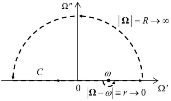Fig. 7.7. Deriving the Kramers-Kronig dispersion relations.

As a result, for our contour \(\ C\), Eq. (49) yields

\[\ f(\omega)=\lim _{r \rightarrow 0} \frac{1}{2 \pi i}\left(\int_{-\infty}^{\omega-r}+\int_{\omega+r}^{+\infty}\right) f(\Omega) \frac{d \Omega}{\Omega-\omega}+\frac{1}{2} f(\omega).,\tag{7.51}\]

where \(\ \Omega \equiv \Omega^{\prime}\) on the real axis (where \(\ \Omega^{\prime \prime}=0\)). Such an integral, excluding a symmetric infinitesimal vicinity of a pole singularity, is called the principal value of the (formally, diverging) integral from \(\ -\infty\) to \(\ +\infty\), and is denoted by the letter P before it.²⁴ Using this notation, subtracting \(\ f(\omega) / 2\) from both parts of Eq. (51), and multiplying them by 2, we get

\[\ f(\omega)=\frac{1}{\pi i} \mathrm{P} \int_{-\infty}^{+\infty} f(\Omega) \frac{d \Omega}{\Omega-\omega}.\tag{7.52}\]

Now plugging into this complex equality the polarization-related difference \(\ f(\omega) \equiv \varepsilon(\omega)-\varepsilon_{0}\) in the form \(\ \left[\varepsilon^{\prime}(\omega)-\varepsilon_{0}\right]+i\left[\varepsilon^{\prime \prime}(\omega)\right]\), and requiring both real and imaginary components of the two sides of Eq. (52) to be equal separately, we get the famous Kramers-Kronig dispersion relations

\[\ \text{Kramers-Kronig dispersion relations}\quad\quad\quad\quad\varepsilon^{\prime}(\omega)=\varepsilon_{0}+\frac{1}{\pi} \mathrm{P} \int_{-\infty}^{+\infty} \varepsilon^{\prime \prime}(\Omega) \frac{d \Omega}{\Omega-\omega}, \quad \varepsilon^{\prime \prime}(\omega)=-\frac{1}{\pi} \mathrm{P} \int_{-\infty}^{+\infty}\left[\varepsilon^{\prime}(\Omega)-\varepsilon_{0}\right] \frac{d \Omega}{\Omega-\omega}.\tag{7.53}\]

We may use the already mentioned fact that \(\ \varepsilon^{\prime}(\omega)\) is always an even function, while \(\ \varepsilon^{\prime \prime}(\omega)\) an odd
function of frequency, to rewrite these relations in the following equivalent form,

\[\ \varepsilon^{\prime}(\omega)=\varepsilon_{0}+\frac{2}{\pi} \mathrm{P} \int_{0}^{+\infty} \varepsilon^{\prime \prime}(\Omega) \frac{\Omega d \Omega}{\Omega^{2}-\omega^{2}}, \quad \varepsilon^{\prime \prime}(\omega)=-\frac{2 \omega}{\pi} \mathrm{P} \int_{0}^{+\infty}\left[\varepsilon^{\prime}(\Omega)-\varepsilon_{0}\right] \frac{d \Omega}{\Omega^{2}-\omega^{2}},\tag{7.54}\]

which is more convenient for most applications, because it involves only physical (positive) frequencies.

Though the Kramers-Kronig relations are “global” in frequency, in certain cases they allow an approximate calculation of dispersion from experimental data for absorption, collected even within a limited (“local”) frequency range. Most importantly, if a medium has a sharp absorption peak at some frequency \(\ \omega_{j}\), we may describe it as

\[\ \varepsilon^{\prime \prime}(\omega) \approx c \delta\left(\omega-\omega_{j}\right)+\text { a more smooth function of } \omega,\tag{7.55}\]

and the first of Eqs. (54) immediately gives

\[\ \varepsilon^{\prime}(\omega) \approx \varepsilon_{0}+\frac{2 c}{\pi} \frac{\omega_{j}}{\omega_{j}^{2}-\omega^{2}}+\text { another smooth function of } \omega\quad\quad\quad\quad\text{Dispersion near an absorption line}\tag{7.56}\]

thus predicting the anomalous dispersion near such a point. This calculation shows that such behavior observed in the Lorentz oscillator model (see Fig. 5) is by no means occasional or model-specific.

Let me emphasize again that the Kramers-Kronig relations (53)-(54) are much more general than the Lorentz model (33), and require only a causal, linear relation (21) between the polarization \(\ P(t)\) with the electric field \(\ E\left(t^{\prime}\right)\).²⁵ Hence, these relations are also valid for the complex functions relating Fourier images of any cause/effect-related pair of variables. In particular, at a measurement of any linear response \(\ r(t)\) of any experimental sample to any external field \(\ f\left(t^{\prime}\right)\), whatever the nature of this response and physics behind it, we may be confident that there is a causal relationship between the variables \(\ r\) and \(\ f\), so that the corresponding complex function \(\ \chi(\omega) \equiv r_{\omega} / f_{\omega}\) does obey the Kramers-Kronig relations. However, it is still important to remember that a linear relationship between the Fourier amplitudes of two variables does not necessarily imply a causal relationship between them.²⁶

---

Reference

⁸ In an isotropic media, the vectors E, P, and hence \(\ \mathbf{D}=\varepsilon_{0} \mathbf{E}+\mathbf{P}\), are all parallel, and for the notation simplicity, I
will drop the vector sign in the following formulas. I am also assuming that P at any point r is only dependent on the electric field at the same point, and hence drop the factor \(\ \exp \{i k z\}\), the same for all variables. This last assumption is valid if the wavelength \(\ \lambda\) is much larger than the elementary media dipole’s size \(\ a\). In most systems of interest, the scale of \(\ a\) is atomic \(\ \left(\sim 10^{-10} \mathrm{~m}\right)\), so that the approximation is valid up to very high frequencies, \(\ \omega \sim c / a \sim 10^{18} \mathrm{~s}^{-1}\), corresponding to hard X-rays.

⁹ The idea of these functions is very similar to that of the spatial Green’s functions (see Sec. 2.10), but with the new twist, due to the causality principle. A discussion of the temporal Green’s functions in application to classical mechanics (which to some extent overlaps with our current discussion) may be found in CM Sec. 5.1.

¹⁰ The first unambiguous observations of dispersion (for the case of light refraction) were described by Sir Isaac Newton in his Optics (1704) – even though this genius has never recognized the wave nature of light!

¹¹ It may be tempting to attribute this effect to wave absorption, i.e. the dissipation of the wave’s energy, but we will see very soon that wave attenuation may be due to different effects as well.

¹² The reader is probably familiar with the most noticeable effect of the dispersion: the difference between that group velocity \(\ \nu_{\mathrm{gr}} \equiv d \omega / d k^{\prime}\), giving the speed of the envelope of a wave packet with a narrow frequency spectrum, and the phase velocity \(\ \nu _{\mathrm{ph}} \equiv \omega / k^{\prime}\) of the component waves. The second-order dispersion effect, proportional to \(\ d^{2} \omega / d^{2} k^{\prime}\), leads to the deformation (gradual broadening) of the envelope itself. Following tradition, these effects are discussed in more detail in the quantum-mechanics part of this series (QM Sec. 2.2), because they are the crucial factor of Schrödinger’s wave mechanics. (See also a brief discussion in CM Sec. 6.3.)

¹³ This example is focused on the frequency dependence of \(\ varepsilon\) rather than \(\ \mu\), because electromagnetic waves interact with “usual” media via their electric field much more than via the magnetic field. Indeed, according to Eq. (7), the magnetic field of the wave is of the order of \(\ E / c\), so that the magnetic component of the Lorentz force (5.10), acting on a non-relativistic particle, \(\ F_{\mathrm{m}} \sim q u B \sim(u / c) q E\), is much smaller than that of its electric component, \(\ F_{\mathrm{e}}=q E\), and may be neglected. However, as will be discussed in Sec. 6, forgetting about the possible dispersion of \(\ \mu(\omega)\) may result in missing some remarkable opportunities for manipulating the waves.

¹⁴ If this point is not absolutely clear, please see CM Sec. 5.1 for a more detailed discussion.

¹⁵ In optics, such behavior is called anomalous dispersion.

¹⁶ See, e.g., QM Chapters 5-6.

¹⁷ For an arbitrary plane wave, the total average power flow may be calculated as an integral of Eq. (42) over all frequencies. By the way, combining this integral and the Poynting theorem (6.111), is it straightforward to prove the following interesting expression for the average electromagnetic energy density of a narrow \(\ (\Delta \omega<<\omega)\) wave packet propagating in an arbitrary dispersive (but linear and isotropic) medium:

\(\ \bar{u}=\frac{1}{2} \int_{\text {packet }}\left\{\frac{d\left[\omega \varepsilon^{\prime}(\omega)\right]}{d \omega} E_{\omega} E_{\omega}^{*}+\frac{d\left[\omega \mu^{\prime}(\omega)\right]}{d \omega} H_{\omega} H_{\omega}^{*}\right\} d \omega .\)

¹⁸ One more convenience of the simple model of a collision-free plasma, which has led us to Eq. (36), is that it may be readily generalized to the case of an additional strong dc magnetic field \(\ \mathbf{B}_{0}\) (much higher than that of the wave) applied in the direction n of wave propagation. It is straightforward (and hence left for the reader) to show that such plasma exhibits the Faraday effect of the polarization plane’s rotation, and hence gives an example of an anisotropic media that violates the Lorentz reciprocity relation (6.121).

¹⁹ These frequencies are an order of magnitude lower than those used for TV and FM-radio broadcasting.

²⁰ Alternatively, according to Eq. (45), it is possible (and in the field of infrared spectroscopy, conventional) to attribute the ac response of a medium at all frequencies to its effective complex conductivity: \(\ \sigma_{\mathrm{ef}}(\omega)\equiv\sigma(\omega)-i \omega \varepsilon(\omega) \equiv-i \omega \varepsilon_{\mathrm{ef}}(\omega)\).

²¹ It may be also derived from the Boltzmann kinetic equation in the so-called relaxation-time approximation (RTA) – see, e.g., SM Sec. 6.2.

²² See, e.g., MA Eq. (15.2).

²³Strictly speaking, this also requires \(\ |f(\Omega)|\) to decrease faster than \(\ \Omega^{-1}\) at the real axis (at \(\ \Omega^{\prime \prime}=0\)), but due to the
inertia of charged particles, this requirement is fulfilled for all realistic models of dispersion – see, e.g., Eq. (36).

²⁴ I am typesetting this symbol in a Roman (upright) font, to avoid any possibility of its confusion with the medium’s polarization.

²⁵ Actually, in mathematics, the relations even somewhat more general than Eqs. (53), valid for an arbitrary analytic function of complex argument, are known at least from 1868 (the Sokhotski-Plemelj theorem).

²⁶ For example, the function \(\ \varphi(\omega) \equiv E_{\omega} / P_{\omega}\), in the Lorentz oscillator model, does not obey the Kramers-Kronig relations. This is evident not only physically, from the fact that \(\ E(t)\) is not a causal function of \(\ P(t)\), but even mathematically. Indeed, Green’s function describing a causal relationship has to tend to zero at small time delays \(\ \theta \equiv t-t^{\prime}\), so that its Fourier image has to tend to zero at \(\ \omega \rightarrow \pm \infty\). This is certainly true for the function \(\ f(\omega)\) given by Eq. (32), but not for the reciprocal function \(\ \varphi(\omega) \equiv 1 / f(\omega) \propto\left(\omega^{2}-\omega_{0}^{2}\right)-2 i \delta \omega\), which diverges at large frequencies.