8.1: Retarded Potentials

Let us start by finding the general solution of the macroscopic Maxwell equations (6.99) in a dispersion-free, linear, uniform, isotropic medium, characterized by frequency-independent, real \(\ \varepsilon\) and \(\ \mu\).¹ The easiest way to perform this calculation is to use the scalar \(\ (\phi)\) and vector (\(\ \mathbf{A}\)) potentials defined by Eqs. (6.7):

\[\ \mathbf{E}=-\nabla \phi-\frac{\partial \mathbf{A}}{\partial t}, \quad \mathbf{B}=\nabla \times \mathbf{A}.\tag{8.1}\]

As was discussed in Sec. 6.8, by imposing upon the potentials the Lorenz gauge condition (6.117),

\[\ \nabla \cdot \mathbf{A}+\frac{1}{\nu^{2}} \frac{\partial \phi}{\partial t}=0, \quad \text { with } \nu^{2} \equiv \frac{1}{\varepsilon \mu},\tag{8.2}\]

which does not affect the fields E and B, the Maxwell equations are reduced to a pair of very similar, simple equations (6.118) for the potentials:

\[\ \nabla^{2} \phi-\frac{1}{\nu^{2}} \frac{\partial^{2} \phi}{\partial t^{2}}=-\frac{\rho}{\varepsilon},\tag{8.3a}\]

\[\ \nabla^{2} \mathbf{A}-\frac{1}{\nu^{2}} \frac{\partial^{2} \mathbf{A}}{\partial t^{2}}=-\mu \mathbf{j}.\tag{8.3b}\]

Let us find the general solution of these equations, for now thinking of the densities \(\ \rho(\mathbf{r}, t)\) and \(\ \mathbf{j}(\mathbf{r}, t)\) of the stand-alone charges and currents as of known functions. (This will not prevent the results from being valid for the cases when \(\ \rho(\mathbf{r}, t)\) and \(\ \mathbf{j}(\mathbf{r}, t)\) should be calculated self-consistently.) The idea of such solution may be borrowed from electro- and magnetostatics. Indeed, for the stationary case \(\ (\partial / \partial t=0)\), the solutions of Eqs. (8.3) are given, by a ready generalization of, respectively, Eqs. (1.38) and (5.28) to a uniform, linear medium:

\[\ \phi(\mathbf{r})=\frac{1}{4 \pi \varepsilon} \int \rho\left(\mathbf{r}^{\prime}\right) \frac{d^{3} r^{\prime}}{\left|\mathbf{r}-\mathbf{r}^{\prime}\right|},\tag{8.4a}\]

\[\ \mathbf{A}(\mathbf{r}) \equiv \frac{\mu}{4 \pi} \int \mathbf{j}\left(\mathbf{r}^{\prime}\right) \frac{d^{3} r^{\prime}}{\left|\mathbf{r}-\mathbf{r}^{\prime}\right|}\tag{8.4b}\]

As we know, these expressions may be derived by, first, calculating the potential of a point source, and then using the linear superposition principle for a system of such sources.

Let us do the same for the time-dependent case, starting from the field induced by a time-dependent point charge at the origin:²

\[\ \rho(\mathbf{r}, t)=q(t) \delta(\mathbf{r}),\tag{8.5}\]

In this case, Eq. (3a) is homogeneous everywhere but the origin:

\[\ \nabla^{2} \phi-\frac{1}{\nu^{2}} \frac{\partial^{2} \phi}{\partial t^{2}}=0, \quad \text { for } r \neq 0.\tag{8.6}\]

Due to the spherical symmetry of the problem, it is natural to look for a spherically-symmetric solution to this equation.³ Thus, we may simplify the Laplace operator correspondingly (as was repeatedly done earlier in this course), so that Eq. (6) becomes

\[\ \left[\frac{1}{r^{2}} \frac{\partial}{\partial r}\left(r^{2} \frac{\partial}{\partial r}\right)-\frac{1}{\nu^{2}} \frac{\partial^{2}}{\partial t^{2}}\right] \phi=0, \quad \text { for } r \neq 0.\tag{8.7}\]

If we now introduce a new variable \(\ \chi \equiv r \phi\), Eq. (7) is reduced to a 1D wave equation

\[\ \left(\frac{\partial^{2}}{\partial r^{2}}-\frac{1}{\nu^{2}} \frac{\partial^{2}}{\partial t^{2}}\right) \chi=0, \quad \text { for } r \neq 0.\tag{8.8}\]

From discussions in Chapter 7,⁴ we know that its general solution may be represented as

\[\ \chi(r, t)=\chi_{\text {out }}\left(t-\frac{r}{\nu}\right)+\chi_{\text {in }}\left(t+\frac{r}{\nu}\right),\tag{8.9}\]

where \(\ \chi_{\text {in }}\) and \(\ \chi_{\text {out }}\) are (so far) arbitrary functions of one variable. The physical sense of \(\ \phi_{\text {out }}=\chi_{\text {out }} / r\) is a spherical wave propagating from our source (located at \(\ r = 0\)) to outer space, i.e. exactly the solution we are looking for. On the other hand, \(\ \phi_{\mathrm{in}}=\chi_{\mathrm{in}} / r\) describes a spherical wave that could be created by some distant spherically-symmetric source, that converges exactly on our charge located at the origin – evidently not the effect we want to consider here. Discarding this term, and returning to \(\ \phi=\chi / r\), we get

\[\ \phi(r, t)=\frac{1}{r} \chi_{\text {out }}\left(t-\frac{r}{\nu}\right), \quad \text { for } r \neq 0.\tag{8.10}\]

In order to calculate the function \(\ \chi_{\text {out }}\), let us consider the solution (10) at distances \(\ r\) so small \(\ (r<<\nu t)\) that the time-derivative term in Eq. (3a), with the right-hand side (5),

\[\ \nabla^{2} \phi-\frac{1}{\nu^{2}} \frac{\partial^{2} \phi}{\partial t^{2}}=-\frac{q(t)}{\varepsilon} \delta(\mathbf{r}),\tag{8.11}\]

is much smaller than the spatial derivative term (which diverges at \(\ r \rightarrow 0\)). Then Eq. (11) is reduced to the electrostatic equation, whose solution (4a), for the source (5), is

\[\ \phi(r \rightarrow 0, t)=\frac{q(t)}{4 \pi \varepsilon r}.\tag{8.12}\]

Now requiring the two solutions, Eqs. (10) and (12), to coincide at \(\ r<<\nu t\), we get \(\ \chi_{\text {out }}(t)=q(t) / 4 \pi \varepsilon r\), so that Eq. (10) becomes

\[\ \phi(r, t)=\frac{1}{4 \pi \varepsilon r} q\left(t-\frac{r}{\nu}\right).\tag{8.13}\]

Just as was repeatedly done in statics, this result may be readily generalized for the arbitrary position \(\ \mathbf{r^{\prime}}\) of the point charge:

\[\ \rho(\mathbf{r}, t)=q(t) \delta\left(\mathbf{r}-\mathbf{r}^{\prime}\right) \equiv q(t) \delta(\mathbf{R}),\tag{8.14}\]

where \(\ R\) is the distance between the field observation point \(\ \mathbf{r}\) and the source position point \(\ \mathbf{r}^{\prime}\), i.e. the length of the vector,

\[\ \mathbf{R} \equiv \mathbf{r}-\mathbf{r}^{\prime},\tag{8.15}\]

connecting these points – see Fig. 1.

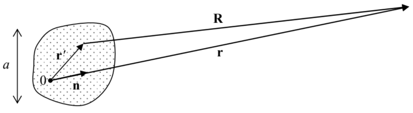Fig. 8.1. Calculating the retarded potentials of a localized source.

Obviously, now Eq. (13) becomes

\[\ \phi(\mathbf{r}, t)=\frac{1}{4 \pi \varepsilon R} q\left(t-\frac{R}{\nu}\right).\tag{8.16}\]

Finally, we may use the linear superposition principle to write, for the arbitrary charge distribution,

\[\ \text{Retarded scalar potential}\quad\quad\quad\quad \phi(\mathbf{r}, t)=\frac{1}{4 \pi \varepsilon} \int \rho\left(\mathbf{r}^{\prime}, t-\frac{R}{\nu}\right) \frac{d^{3} r^{\prime}}{R},\tag{8.17a}\]

where the integration is extended over all charges of the system under analysis. Acting absolutely similarly, for the vector potential we get⁵

\[\ \text{Retarded vector potential}\quad\quad\quad\quad \mathbf{A}(\mathbf{r}, t)=\frac{\mu}{4 \pi} \int \mathbf{j}\left(\mathbf{r}^{\prime}, t-\frac{R}{\nu}\right) \frac{d^{3} r^{\prime}}{R}.\tag{8.17b}\]

(Now nothing prevents the functions \(\ \rho(\mathbf{r}, t)\) and \(\ {\boldsymbol{j}}(\mathbf{r}, t)\) from satisfying the continuity equation.)

The solutions expressed by Eqs. (17) are traditionally called the retarded potentials, the name signifying the fact that the observed fields are “retarded” (in the meaning “delayed”) in time by \(\ \Delta t=R / \nu\) relative to the source variations – physically, because of the finite speed \(\ \nu\) of the electromagnetic wave propagation. These solutions are so important that they deserve at least a couple of general remarks.

First, very remarkably, these simple expressions are exact solutions of the macroscopic Maxwell equations (in a uniform, linear, dispersion-free) medium for an arbitrary distribution of stand-alone charges and currents. They also may be considered as the general solutions of these equations, provided that the integration is extended over all field sources in the Universe – or at least in its part that affects our observations.

Second, due to the mathematical similarity of the microscopic and macroscopic Maxwell equations, Eqs. (17) are valid, with the coefficient replacement \(\ \varepsilon \rightarrow \varepsilon_{0}\) and \(\ \mu \rightarrow \mu_{0}\), for the exact, rather than the macroscopic fields, provided that the functions \(\ \rho(\mathbf{r}, t)\) and \(\ \mathbf{j}(\mathbf{r}, t)\) describe not only stand-alone but all charges and currents in the system. (Alternatively, this statement may be formulated as the validity of Eqs. (17), with the same coefficient replacement, in free space.)

Finally, Eqs. (17) may be plugged into Eqs. (1), giving (after an explicit differentiation) the so-called Jefimenko equations for fields E and B – similar in structure to Eqs. (17), but more cumbersome. Conceptually, the existence of such equations is good news, because they are free from the gauge ambiguity pertinent to the potentials \(\ \phi\) and A. However, the practical value of these explicit expressions for the fields is not too high: for all applications I am aware of, it is easier to use Eqs. (17) to calculate the particular expressions for the potentials first, and only then calculate the fields from Eqs. (1). Let me now present an (apparently, the most important) example of this approach.

---

Reference

¹ When necessary (e.g., at the discussion of the Cherenkov radiation in Sec. 10.5), it will be not too hard to generalize these results to a dispersive medium.

² Admittedly, this expression does not satisfy the continuity equation (4.5), but this deficiency will be corrected imminently, at the linear superposition stage – see Eq. (17) below.

³ Let me confess that this is not the general solution to Eq. (6). For example, it does not describe the possible waves created by other sources, that pass by the considered charge \(\ q(t)\). However, such fields are irrelevant for our current task: to calculate the field created by the charge \(\ q(t)\). The solution becomes general when it is integrated (as it will be) over all charges of interest.

⁴ See also CM Sec. 6.3.

⁵ As should be clear from the analogy of Eqs. (17) with their stationary forms (4), which were discussed, respectively, in Chapters 1 and 5, in the Gaussian units the retarded potential formulas are valid with the coefficient \(\ 1 / 4 \pi\) dropped in Eq. (17a), and replaced with \(\ 1 / c\) in Eq. (17b).