4.6: Trajectories in the Complex Plane

Last updated
Save as PDF

Page ID: 34538

\( \newcommand{\vecs}[1]{\overset { \scriptstyle \rightharpoonup} {\mathbf{#1}} } \) \( \newcommand{\vecd}[1]{\overset{-\!-\!\rightharpoonup}{\vphantom{a}\smash {#1}}} \)\(\newcommand{\id}{\mathrm{id}}\) \( \newcommand{\Span}{\mathrm{span}}\) \( \newcommand{\kernel}{\mathrm{null}\,}\) \( \newcommand{\range}{\mathrm{range}\,}\) \( \newcommand{\RealPart}{\mathrm{Re}}\) \( \newcommand{\ImaginaryPart}{\mathrm{Im}}\) \( \newcommand{\Argument}{\mathrm{Arg}}\) \( \newcommand{\norm}[1]{\| #1 \|}\) \( \newcommand{\inner}[2]{\langle #1, #2 \rangle}\) \( \newcommand{\Span}{\mathrm{span}}\) \(\newcommand{\id}{\mathrm{id}}\) \( \newcommand{\Span}{\mathrm{span}}\) \( \newcommand{\kernel}{\mathrm{null}\,}\) \( \newcommand{\range}{\mathrm{range}\,}\) \( \newcommand{\RealPart}{\mathrm{Re}}\) \( \newcommand{\ImaginaryPart}{\mathrm{Im}}\) \( \newcommand{\Argument}{\mathrm{Arg}}\) \( \newcommand{\norm}[1]{\| #1 \|}\) \( \newcommand{\inner}[2]{\langle #1, #2 \rangle}\) \( \newcommand{\Span}{\mathrm{span}}\)\(\newcommand{\AA}{\unicode[.8,0]{x212B}}\)

If we have a function \(z(t)\) which takes a real input \(t\) and outputs a complex number \(z\), it is often useful to plot a curve in the complex plane called the “parametric trajectory” of \(z\). Each point on this curve indicates the value of \(z\) for a particular value of \(t\). We will give a few examples below.

First, consider \[z(t) = e^{i\omega t}, \quad \omega \in \mathbb{R}.\] The trajectory is a circle in the complex plane, centered at the origin and with radius 1:

To see why, observe that the function has the form \(z(t) = r(t)\,e^{i\theta(t)}\), which has magnitude \(r(t) = 1\), and argument \(\theta(t) = \omega t\) varying proportionally with \(t\). If \(\omega\) is positive, the argument increases with \(t\), so the trajectory is counter-clockwise. If \(\omega\) is negative, the trajectory is clockwise.

Next, consider \[z(t) = e^{(\gamma + i \omega) t},\] where \(\gamma,\omega \in \mathbb{R}.\) For \(\gamma = 0\), this reduces to the previous example. For \(\gamma \ne 0\), the trajectory is a spiral:

To see this, we again observe that this function can be written in the form \[z(t) = r(t) \;e^{i\theta(t)},\] where \(r(t) = e^{\gamma t}\) and \(\theta = \omega t.\) The argument varies proportionally with \(t\), so the trajectory loops around the origin. The magnitude increases with \(t\) if \(\gamma\) is positive, and decreases with \(t\) if \(\gamma\) is negative. Thus, for instance, if \(\gamma\) and \(\omega\) are both positive, then the trajectory is an anticlockwise spiral moving outwards from the origin. Try checking how the trajectory behaves when the signs of \(\gamma\) and/or \(\omega\) are flipping.

Finally, consider \[z(t) = \frac{1}{\alpha t + \beta}, \quad \alpha, \beta \in \mathbb{C}.\] This trajectory is a circle which passes through the origin, as shown below:

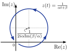
Showing this requires a bit of ingenuity, and is left as an exercise. This is an example of something called a Möbius transformation.