5.3: General Solution for the Damped Harmonic Oscillator

For now, suppose \(\omega_0 \ne \gamma\). In the previous section, we found two classes of specific solutions, with complex frequencies \(\omega_+\) and \(\omega_-\): \[z_+(t) = e^{-i\omega_+ t} \;\;\mathrm{and}\;\; z_-(t) = e^{-i\omega_- t}, \;\;\mathrm{where} \;\;\; \omega_\pm = -i\gamma \pm \sqrt{\omega_0^2 - \gamma^2}.\] A general solution can be found by constructing a linear superposition of these solutions: \[\begin{align} z(t) &= \psi_+ e^{-i\omega_+ t} + \psi_- e^{-i\omega_- t} \\ &= \psi_+ \, \exp\left[\left(-\gamma - i \sqrt{\omega_0^2 - \gamma^2}\right)t\right] \; +\; \psi_- \, \exp\left[\left(-\gamma +i\sqrt{\omega_0^2 - \gamma^2}\right)t\right]. \label{gensol}\end{align}\] This contains two undetermined complex parameters, \(\psi_+\) and \(\psi_-\). These are independent parameters since they are coefficients multiplying different functions (the functions are different because \(\omega_0 \ne \gamma\) implies that \(\omega_+ \ne \omega_-\)).

To obtain the general solution to the real damped harmonic oscillator equation, we must take the real part of the complex solution. The result can be further simplified depending on whether \(\omega_0^2 - \gamma^2\) is positive or negative. This leads to under-damped solutions or over-damped solutions, as discussed in the following subsections.

What if \(\omega_0 = \gamma\)? In this instance, \(\omega_+ = \omega_-\), which means that \(\psi_+\) and \(\psi_-\) aren’t independent parameters. Therefore, the above equation for \(z(t)\) isn’t a valid general solution! We will discuss how to handle this case Section 5.3.

Under-damped motion

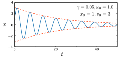
For \(\omega_0 > \gamma\), let us define, for convenience, \[\Omega = \sqrt{\omega_0^2 - \gamma^2}.\] Then we can simplify the real solution as follows: \[\begin{align} x(t) &= \mathrm{Re}\left[z(t)\right] \\ &= e^{-\gamma t} \; \mathrm{Re}\left[\psi_+ \, e^{-i \Omega t} \,+\, \psi_- \, e^{i\Omega t}\right] \\ &= e^{-\gamma t} \left[ A\cos\left(\Omega t\right) + B \sin\left(\Omega t\right)\right], \;\;\mathrm{where}\;\; A, B \in \mathbb{R} \label{underdamped-sol}\end{align}\] With a bit of algebra, we can show that \[A = \mathrm{Re}\left[\psi_+ + \psi_-\right], \quad B = \mathrm{Im}\left[\psi_+ - \psi_-\right].\] This is called an under-damped solution. The coefficients \(A\) and \(B\) act as two independent real parameters, so this is a valid general solution for the real damped harmonic oscillator equation. Using the trigonometric formulas, the solution can be equivalently written as \[x(t) = C e^{-\gamma t} \cos\left[\Omega t + \Phi\right],\] with the parameters \(C = \sqrt{A^2 + B^2}\) and \(\Phi = - \tan^{-1}\left[B/A\right]\).

As shown below, the trajectory is an oscillation whose amplitude decreases with time. The decrease in the amplitude can be visualized using a smooth “envelope” given by \(\pm C e^{-\gamma t}\), which is drawn with dashes in the figure. Inside this envelope, the trajectory oscillates with frequency \(\Omega = \sqrt{\omega_0^2 - \gamma^2}\), which is slightly less than the natural frequency of oscillation \(\omega_0\).

Figure \(\PageIndex{1}\)

Over-damped motion

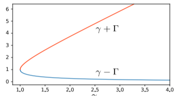
For \(\omega_0 < \gamma\), the square root term is imaginary. It is convenient to define \[\Gamma = \sqrt{\gamma^2 - \omega_0^2} \quad \Rightarrow \quad \sqrt{\omega_0^2 - \gamma^2} = i \Gamma.\] Then the real solution simplifies in a different way: \[\begin{align} x(t) = \mathrm{Re}\left[z(t)\right] &= \mathrm{Re}\left[\psi_+ e^{\left(-\gamma + \Gamma\right)t} + \psi_- e^{\left(-\gamma - \Gamma\right)t} \right] \\ &= C_+ e^{-(\gamma - \Gamma) t} + C_- e^{-(\gamma + \Gamma) t}, \label{overdamped-sol}\end{align}\] where \[C_\pm = \mathrm{Re}[\psi_\pm].\] This is called an over-damped solution. It consists of two terms, both exponentially decaying in time, with \((\gamma-\Gamma)\) and \((\gamma + \Gamma)\) serving as the decay rates. Note that both decay rates are positive real numbers, because \(\Gamma < \gamma\) from the definition of \(\Gamma\). Also, note that \((\gamma - \Gamma)\) decreases with \(\gamma\), whereas \((\gamma + \Gamma)\) increases with \(\gamma\), as shown below:

Figure \(\PageIndex{2}\)

The plot below shows trajectory of the over-damped oscillator:

Figure \(\PageIndex{3}\)

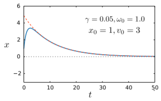
The red dashes show the limiting curve determined by the decay rate \((\gamma - \Gamma)\). The other decay rate, \((\gamma + \Gamma)\), corresponds to a faster-decaying exponential, so at long times the second term in Eq. \(\eqref{overdamped-sol}\) becomes negligible compared to the first term. Then the solution approaches the limit \[x(t) \approx C_+ e^{-(\gamma - \Gamma) t} \qquad (\mathrm{for}~\mathrm{large}~t). \label{overdamped-long-t}\] Interestingly, since \((\gamma-\Gamma)\) is a decreasing function of \(\gamma\), the stronger the damping, the slower the decay rate at long times. This is the opposite of what happens in the under-damped regime!

Why does this happen? In the over-damped regime, the motion of the oscillator is dominated by the damping force rather than the spring force; as the oscillator tries to return to its equilibrium position \(x = 0\), the damping acts against this motion. Hence, the stronger the damping, the slower the decay to equilibrium. This contrasts sharply with the Section 5.3, where the spring force dominates the damping force. In that case, stronger damping speeds up the decay to equilibrium, by causing the kinetic energy of the oscillation to dissipate more rapidly.

Critical damping

Critical damping occurs when \(\omega_0 = \gamma\). Under this special condition, Eq. \(\eqref{gensol}\) reduces to \[z(t) = \left(\psi_+ + \psi_-\right) e^{-\gamma t}.\] This has only one independent complex parameter, i.e. the parameter \((\psi_+ + \psi_-)\). Therefore, it cannot be a general solution for the complex damped harmonic oscillator equation, which is still a second-order ODE.

We will not go into detail here regarding the procedure for finding the general solution for the critically-damped oscillator, leaving it as an Section 5.5 for the interested reader. Basically, the procedure is to Taylor expand the solution on either side of the critical point, and then show that there is a solution of the form \[z(t) = \left(A + B t\right)\, e^{-\gamma t}, \label{critical-sol}\] which contains the desired two independent parameters.

The critically-damped solution contains an exponential decay constant of \(\gamma\), which is the same as the decay constant for the envelope function in the under-damped regime [Eq. \(\eqref{underdamped-sol}\)], and smaller than the long-time decay constants in the over-damped regime [Eq. \(\eqref{overdamped-long-t}\)]. Hence, we can regard the critically-damped solution as the fastest-decaying non-oscillatory solution.

This feature of critical damping is employed in many engineering contexts, the most familiar being automatic door closers. If the damping is too weak or the spring force is too strong (under-damped), the door will slam shut, whereas if the damping is too strong or the spring force is too weak (under-damping), the door takes unnecessarily long to close. Hence, door closers must be tuned to a “sweet spot” corresponding to the critical damping point.