9.1: Contour Integrals

Recall that for a real function \(f(x)\), the definite integral from \(x=a\) to \(x=b\) is the area under the curve between those two points. As discussed in Chapter 3, the integral can be expressed as a limit expression: we divide the interval into \(N\) segments of width \(\Delta x\), take the sum of \(\Delta x\, f(x_n)\), and go to the \(N \rightarrow \infty\) limit: \[\int_a^b dx\; f(x) \;=\; \lim_{N \rightarrow 0} \, \sum_{n=0}^{N} \Delta x\; f(x_n), \;\;\;\mathrm{where}\;\;\;x_n = a + n\Delta x, \;\;\Delta x = \frac{b-a}{N}.\] Now suppose \(f\) is a complex function of a complex variable. 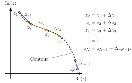A straight-foward way to define the integral of \(f(z)\) is to adopt an analogous expression: \[\lim_{N \rightarrow 0} \, \sum_{n=0}^{N} \Delta z\; f(z_n)\] But there’s a conceptual snag: since \(f\) takes complex inputs, the values of \(z_n\) need not lie along the real line. In general, the complex numbers \(z_n\) form a set of points in the complex plane. To accommodate this, we can imagine chaining together a sequence of points \(z_1, z_2, \dots, z_N\), separated by displacements \(\Delta z_1, \Delta z_2, \Delta z_3, \dots, \Delta z_{N-1}\):

Figure \(\PageIndex{1}\)

Then the sum we are interested in is \[\sum_{n=1}^{N-1} \Delta z_n\; f(z_n) \;=\; \Delta z_1\, f(z_1) + \Delta z_2\, f(z_2) + \cdots + \Delta z_{N-1}\, f(z_{N-1}).\] In the limit \(N \rightarrow \infty\), each displacement \(\Delta z_{n}\) becomes infinitesimal, and the sequence of points \(\{z_1, z_2, \dots, z_N\}\) becomes a continuous trajectory in the complex plane (see Section 4.6). Such a trajectory is called a contour. Let us denote a given contour by an abstract symbol, such as \(\Gamma\). Then the contour integral over \(\Gamma\) is defined as \[\int_\Gamma \, f(z)\, dz = \lim_{N \rightarrow \infty} \sum_{n=1}^{N-1} \Delta z_n\; f(z_n).\] The symbol \(\Gamma\) in the subscript of the integral sign indicates that the integral takes place over the contour \(\Gamma\). When defining a contour integral, it is always necessary to specify which contour we are integrating over. This is analogous to specifying the end-points of the interval over which to perform a definite real integral. In the complex case, the integration variable \(z\) lies in a two-dimensional plane (the complex plane), not a line; therefore we cannot just specify two end-points, and must specify an entire contour.

Also, note that in defining a contour \(\Gamma\) we must specify not just a curve in the complex plane, but also the direction along which to traverse the curve. If we integrate along the same curve in the opposite direction, the value of the contour integral switches sign (this is similar to swapping the end-points of a definite real integral).

Note

A contour integral generally cannot be interpreted as the area under a curve, the way a definite real integral can. In particular, the contour should not be mistakenly interpreted the graph of the integrand! Always remember that in a contour integral, the integrand \(f(z)\) and the integration variable \(z\) are both complex numbers.

Moreover, the concept of an indefinite integral cannot be usefully generalized to the complex case.

Contour integral along a parametric curve

Simple contour integrals can be calculated by parameterizing the contour. Consider a contour integral \[\int_\Gamma \, dz \; f(z),\] where \(f\) is a complex function of a complex variable and \(\Gamma\) is a given contour. As discussed in Section 4.6, we can describe a trajectory in the complex plane by a complex function of a real variable, \(z(t)\): \[\Gamma \equiv \Big\{z(t) \;\Big|\; t_1 < t < t_2\Big\}, \quad \mathrm{where}\;\; t \in \mathbb{R}, \,z(t) \in \mathbb{C}.\] The real numbers \(t_1\) and \(t_2\) specify two complex numbers, \(z(t_1)\) and \(z(t_2)\), which are the end-points of the contour. The rest of the contour consists of the values of \(z(t)\) between those end-points. Provided we can parameterize \(\Gamma\) in such a manner, the complex displacement \(dz\) in the contour integral can be written as \[dz \rightarrow dt\, \frac{dz}{dt}.\] Then we can express the contour integral over \(\Gamma\) as a definite integral over \(t\): \[\int_\Gamma dz\; f(z) = \int_{t_1}^{t_2} \; dt\; \frac{dz}{dt}\, f\big(z(t)\big).\] This can then be calculated using standard integration techniques. A simple example is given in the next section.

A contour integral over a circular arc

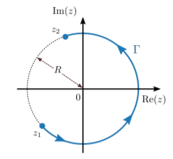
Let us use the method of parameterizing the contour to calculate the contour integral \[\int_{\Gamma[R, \theta_1,\theta_2]} dz\; z^n,\; n\in\mathbb{Z},\] where the trajectory \(\Gamma[R, \theta_1,\theta_2]\) consists of a counter-clockwise arc of radius \(R > 0\), from the point \(z_1 = R e^{i\theta_1}\) to the point \(z_2 = R e^{i\theta_2}\), as shown in the figure below:

Figure \(\PageIndex{2}\)

We can parameterize the contour as follows: \[\Gamma[R, \theta_1,\theta_2] = \big\{z(\theta) \;\big|\; \theta_1 \le \theta \le \theta_2\big\}, \quad \mathrm{where}\;\, z(\theta) = R e^{i\theta}.\] Then the contour integral can be converted into an integral over the real parameter \(\theta\): \[\begin{align} \int_{\Gamma[R, \theta_1,\theta_2]} dz\; z^n &= \int_{\theta_1}^{\theta_2} d\theta \; z^n \; \frac{dz}{d\theta} \\ &= \int_{\theta_1}^{\theta_2} d\theta \; \left( Re^{i\theta}\right)^n\, \left(iR\, e^{i\theta}\right) \\ &= i R^{n+1} \, \int_{\theta_1}^{\theta_2} d\theta \; e^{i(n+1)\theta}.\end{align}\] To proceed, there are two cases that we must treat separately. First, for \(n \ne -1\), \[\int_{\theta_1}^{\theta_2} d\theta \; e^{i(n+1)\theta} = \left[\frac{e^{i(n+1)\theta}}{i(n+1)}\right]_{\theta_1}^{\theta_2} = \frac{e^{i(n+1)\theta_2} - e^{i(n+1)\theta_1}}{i(n+1)}.\] Second, we have the case \(n = -1\). This cannot be handled by the above equations, since the factor of \(n + 1\) in the denominator would vanish. Instead, \[\int_{\theta_1}^{\theta_2} d\theta \; \left[e^{i(n+1)\theta} \right]_{n=-1} \; = \int_{\theta_1}^{\theta_2} d\theta \;=\; \theta_2 - \theta_1.\] Putting the two cases together, we arrive at the result \[\int_{\Gamma[\theta_1,\theta_2]} dz\; z^n = \left\{\begin{array}{ll}i(\theta_2 - \theta_1), & \mathrm{if}\;n = -1 \\ \displaystyle R^{n+1}\frac{e^{i(n+1)\theta_2} - e^{i(n+1)\theta_1}}{n+1},&\mathrm{if}\;n\ne -1.\end{array}\right. \label{arcresult}\] The case where \(\theta_2 = \theta_1 + 2\pi\) is of particular interest. Here, \(\Gamma\) forms a complete loop, and the result simplifies to \[\oint_{\Gamma} dz\; z^n = \left\{\begin{array}{ll}2\pi i, & \mathrm{if}\;n = -1 \\ \displaystyle 0,&\mathrm{if}\;n\ne -1,\end{array}\right. \label{simpleloop}\] which is independent of \(R\) as well as the choice of \(\theta_1\) and \(\theta_2\). (Here, the special integration symbol \(\oint\) is used to indicate that the contour integral is taken over a loop.) Eq. \(\eqref{simpleloop}\) is a very important result that we will make ample use of later.

By the way, what if \(n\) is not an integer? In that case, the integrand \(z^n\) is a multi-valued operation (see Chapter 8), whereas the definition of a contour integral assumes the integrand is a well-defined function. To get around this problem, we can specify a branch cut and perform the contour integral with any of the branches of \(z^n\) (this is fine since the branches are well-defined functions). So long as the branch cut avoids intersecting with the contour \(\Gamma\), the result \(\eqref{arcresult}\) remains valid. However, \(\Gamma\) cannot properly be taken along a complete loop, as that would entail crossing the branch cut.