9.3: Poles

In the previous section, we referred to situations where \(f(z)\) is non-analytic at discrete points. “Discrete”, in this context, means that each point of non-analyticity is surrounded by a finite region over which \(f(z)\) is analytic, isolating it from other points of non-analyticity. Such situations commonly arise from functions of the form \[f(z) \approx \frac{A}{(z-z_0)^n}, \quad \mathrm{where}\;\; n\in\{1,2,3,\dots\}.\] For \(z = z_0\), the function is non-analytic because its value is singular. Such a function is said to have a pole at \(z_0\). The integer \(n\) is called the order of the pole.

Residue of a simple pole

Poles of order 1 are called simple poles, and they are of special interest. Near a simple pole, the function has the form \[f(z) \approx \frac{A}{z-z_0}.\] In this case, the complex numerator \(A\) is called the residue of the pole (so-called because it’s what’s left-over if we take away the singular factor corresponding to the pole.) The residue of a function at a point \(z_0\) is commonly denoted \(\mathrm{Res}[f(z_0)]\). Note that if a function is analytic at \(z_0\), then \(\mathrm{Res}[f(z_0)] = 0\).

Example \(\PageIndex{1}\)

Consider the function \[f(z) = \frac{5}{i-3z}.\] To find the pole and residue, divide the numerator and denominator by \(-3\): \[f(z) = \frac{-5/3}{z-i/3}.\] Thus, there is a simple pole at \(z = i/3\) with residue \(-5/3\).

Example \(\PageIndex{2}\)

Consider the function \[f(z) = \frac{z}{z^2 + 1}.\] To find the poles and residues, we factorize the denominator: \[f(z) = \frac{z}{(z+i)(z-i)}.\] Hence, there are two simple poles, at \(z = \pm i\).

To find the residue at \(z = i\), we separate the divergent part to obtain \[\begin{align} f(z) &= \frac{\left(\frac{z}{z+i}\right)}{z-i} \\ \Rightarrow\quad \mathrm{Res}\big[\,f(z)\,\big]_{z=i} &= \left[\frac{z}{z+i}\right]_{z=i} = 1/2. \end{align}\] Similarly, for the other pole, \[\mathrm{Res}\big[\,f(z)\,\big]_{z=-i} = \left[\frac{z}{z-i}\right]_{z=-i} = 1/2.\]

The residue theorem

In Section 9.1, we used contour parameterization to calculate \[\oint_{\Gamma} \frac{dz}{z} = 2\pi i,\] where \(\Gamma\) is a counter-clockwise circular loop centered on the origin. This holds for any (non-zero) loop radius. By combining this with the results of Section 9.2, we can obtain the residue theorem:

Theorem \(\PageIndex{1}\)

For any analytic function \(f(z)\) with a simple pole at \(z_0\), \[\oint_{\Gamma[z_0]} dz \; f(z) = \pm 2\pi i \, \mathrm{Res}\big[\,f(z)\,\big]_{z = z_0},\] where \(\Gamma[z_0]\) denotes an infinitesimal loop around \(z_0\). The \(+\) sign holds for a counter-clockwise loop, and the \(-\) sign for a clockwise loop.

By combining the residue theorem with the results of the last few sections, we arrive at a technique for integrating a function \(f(z)\) over a loop \(\Gamma\), called the calculus of residues:

1. Identify the poles of \(f(z)\) in the domain enclosed by \(\Gamma\).

2. Check that these are all simple poles, and that \(f(z)\) has no other non-analytic behaviors (e.g. branch cuts) in the enclosed region.

3. Calculate the residue, \(\mathrm{Res}[f(z_n)]\), at each pole \(z_n\).

4. The value of the loop integral is \[\oint_\Gamma dz\; f(z) = \pm 2\pi i \sum_n \mathrm{Res}\big[\,f(z)\,\big]_{z = z_n}.\]The plus sign holds if \(\Gamma\) is counter-clockwise, and the minus sign if it is clockwise.

Example of the calculus of residues

Consider \[f(z) = \frac{1}{z^2 + 1}.\] This can be re-written as \[f(z) = \frac{1}{(z + i)\,(z-i)}.\] By inspection, we can identify two poles: one at \(+i\), with residue \(1/2i\), and the other at \(-i\), with residue \(-1/2i\). The function is analytic everywhere else.

Suppose we integrate \(f(z)\) around a counter-clockwise contour \(\Gamma_1\) that encloses only the pole at \(+i\), as indicated by the blue curve in the figure below:

Figure \(\PageIndex{1}\)

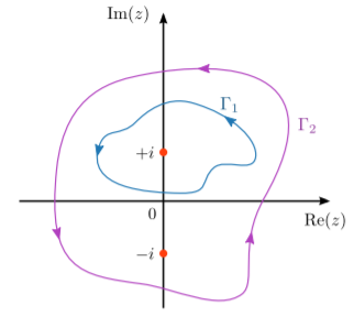
According to the residue theorem, the result is \[\begin{align} \oint_{\Gamma_1}dz \; f(z) &= 2\pi i\, \mathrm{Res}\big[\,f(z)\,\big]_{z = i} \\ &= 2\pi i \cdot \frac{1}{2i} \\& = \pi.\end{align}\] On the other hand, suppose we integrate around a contour \(\Gamma_2\) that encloses both poles, as shown by the purple curve. Then the result is \[\oint_{\Gamma_2}dz \; f(z) = 2\pi i \cdot \left[\frac{1}{2i} - \frac{1}{2i}\right] = 0.\]