9.2: Cauchy's Integral Theorem

A loop integral is a contour integral taken over a loop in the complex plane; i.e., with the same starting and ending point. In Section 9.1, we encountered the case of a circular loop integral. More generally, however, loop contours do not be circular but can have other shapes.

Loop integrals play an important role in complex analysis. This importance stems from the following property, known as Cauchy’s integral theorem:

Theorem \(\PageIndex{1}\)

If \(f(z)\) is analytic everywhere inside a loop \(\Gamma\), then \(\displaystyle\oint_\Gamma dz\; f(z) = 0.\)

Proof of Cauchy’s integral theorem

Cauchy’s integral theorem can be derived from Stokes’ theorem, which states that for any differentiable vector field \(\vec{A}(x,y,z)\) defined within a three-dimensional space, its line integral around a loop \(\Gamma\) is equal to the flux of its curl through any surface enclosed by the loop. Mathematically, this is stated as \[\oint_\Gamma \vec{d\ell} \cdot \vec{A} = \int_{S(\Gamma)} d^2r \; \hat{n} \cdot \left(\nabla \times \vec{A}\right),\] where \(S(\Gamma)\) denotes a two-dimensional surface enclosed by the loop \(\Gamma\), and \(\hat{n}\) denotes a normal vector sticking out of the surface at each integration point.

We only need the 2D version of Stokes’ theorem, in which both the loop \(\Gamma\) and the enclosed surface \(S(\Gamma)\) are restricted to the \(x\mathrm{-}y\) plane, and \(\vec{A}(x,y)\) likewise has no \(z\) component. Then Stokes’ theorem simplifies to \[\oint_\Gamma \vec{d\ell} \cdot \vec{A} = \int\!\!\!\int_{S(\Gamma)}\! dx \,dy \; \left(\frac{\partial A_y}{\partial x} - \frac{\partial A_x}{\partial y}\right).\]

Now consider a loop integral \[\oint_\Gamma dz \; f(z),\] where \(\Gamma\) is a loop trajectory and \(f(z)\) is some analytic function that is analytic in the domain \(S(\Gamma)\). Let us decompose \(f\) into its real and imaginary parts, \[f(x+iy) = u(x,y) + iv(x,y).\] The analyticity of \(f\) implies that the real functions \(u\) and \(v\) are differentiable and obey the Cauchy-Riemann equations. Now we can manipulate the loop integral as follows: \[\begin{align} \oint_\Gamma dz \, f(z) &= \oint_\Gamma \left(dx + i dy\right) \; \left(u + i v\right) \\ &= \oint_\Gamma \Bigg(dx\, (u+iv) + dy\, (iu - v) \Bigg) \\ &= \oint_\Gamma \begin{bmatrix}dx\\dy\end{bmatrix} \cdot \begin{bmatrix}u + i v \\ iu - v\end{bmatrix} \\ &= \oint_\Gamma \vec{d\ell} \cdot \vec{A}.\end{align}\] The last expression is a line integral involving the complex vector field \[\vec{A}(x,y) = \begin{bmatrix}u(x,y) + i v(x,y) \\ iu(x,y) - v(x,y)\end{bmatrix}.\] Using Stokes’ theorem in 2D, we convert this into the area integral \[\begin{align} \int\!\!\!\int_{S(\Gamma)} dx \,dy \; \left(\frac{\partial A_y}{\partial x} - \frac{\partial A_x}{\partial y}\right) &= \int\!\!\!\int_{S(\Gamma)} dx \,dy \; \left[\left(i\frac{\partial u}{\partial x} - \frac{\partial v}{\partial x}\right) - \left(\frac{\partial u}{\partial y} + i \frac{\partial v}{\partial y}\right)\right] \\ &= \int\!\!\!\int_{S(\Gamma)} dx \,dy \; \left[- \left(\frac{\partial v}{\partial x} + \frac{\partial u}{\partial y} \right) + i\left(\frac{\partial u}{\partial x} - \frac{\partial v}{\partial y}\right)\right].\end{align}\] On the last line, the two terms in parenthesis are both zero because, according to the Cauchy-Riemann equations, \[\frac{\partial u}{\partial x} = \frac{\partial v}{\partial y}\;\;\mathrm{and}\;\; \frac{\partial u}{\partial y} = -\frac{\partial v}{\partial x}.\] Hence, the loop integral is zero. Q.E.D.

Consequences of Cauchy’s integral theorem

If the integrand \(f(z)\) is non-analytic somewhere inside the loop, Cauchy’s integral theorem does not apply, and the loop integral need not vanish. In particular, suppose \(f(z)\) vanishes at one or more discrete points inside the loop, \(\{z_1, z_2, \dots\}\). Then we can show that \[\oint_\Gamma dz\; f(z) \,=\, \sum_{n} \oint_{z_n} dz\; f(z),\] where \(\oint_{z_n}\) denotes an integral over a loop of infinitesimal radius around the \(n\)-th point of non-analyticity, in the same direction (i.e., clockwise or counter-clockwise) as \(\Gamma\).

The proof of this result is based on the figure below. The red loop, \(\Gamma\), is the contour we want to integrate over. The integrand is analytic throughout the enclosed area except at several discrete points, say \(\{z_1, z_2, z_3\}\).

Figure \(\PageIndex{1}\)

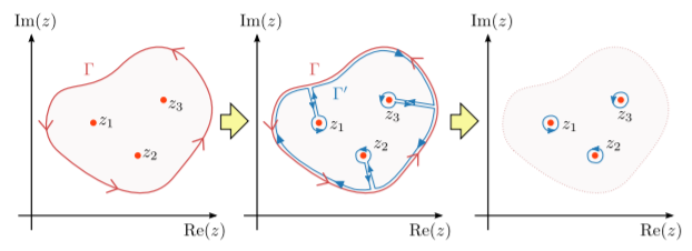
Let us define a new loop contour, \(\Gamma'\), shown by the blue loop. It follows the same curve as \(\Gamma\) but with the following differences: (i) it circles in the opposite direction from \(\Gamma\), (ii) it contains tendrils that extend from the outer curve to each point of non-analyticity, and (iii) each tendril is attached to an infinitesimal loop encircling a point of non-analyticity.

The loop \(\Gamma'\) encloses no points of non-analyticity, so Cauchy’s integral theorem says that the integral over it is zero. But the contour integral over \(\Gamma'\) can be broken up into three pieces: (i) the part that follows \(\Gamma\) but in the opposite direction, (ii) the tendrils, and (iii) the infinitesimal inner loops: \[\begin{align} \oint_{\Gamma'}& dz\; f(z) \;\;= \;\; 0 \quad (\mathrm{by}\;\mathrm{Cauchy's}\;\mathrm{Integral}\;\mathrm{Theorem}) \\ &= \int_{\mathrm{big}\,\mathrm{loop}} dz\; f(z) + \int_{\mathrm{tendrils}} dz\; f(z) +\; \;\sum_{\mathrm{small~loop}~n}\;\; \oint_{z_n} dz\; f(z)\end{align}\] The first term is equal to the negative of \(\oint_\Gamma dz \, f(z)\), since it follows a contour that is just like \(\Gamma\) except going the other way. The second term is zero, because each tendril consists of two contours taken in opposite directions, which cancel. Thus, the above equation reduces to \[\oint_\Gamma dz\; f(z) \,=\, \sum_n \oint_{z_n} dz\; f(z).\] The loop contour integral over \(\Gamma\) is equal to the sum of infinitesimal loop contour integrals encircling each point of non-analyticity. Notably, each of the infinitesimal loops circles in the same direction as \(\Gamma\) (e.g., counter-clockwise in the above figure).

Another way of thinking about this is that Cauchy’s integral theorem says regions of analyticity don’t count towards the value of a loop integral. Hence, we can contract a loop across any domain in which \(f(z)\) is analytic, until the contour becomes as small as possible. This contraction replaces \(\Gamma\) with a discrete set of infinitesimal loops enclosing the points of non-analyticity.