8.2: Sparse Matrix Formats

8.2.1 List of Lists (LIL)

The List of Lists sparse matrix format (which is, for some unknown reason, abbreviated as LIL rather than LOL) is one of the simplest sparse matrix formats. It is shown schematically in the figure below. Each non-zero matrix row is represented by an element in a kind of list structure called a "linked list". Each element in the linked list records the row number, and the column data for the matrix entries in that row. The column data consists of a list, where each list element corresponds to a non-zero matrix element, and stores information about (i) the column number, and (ii) the value of the matrix element.

Figure \(\PageIndex{1}\): A sparse matrix and its representation in List-of-Lists (LIL) format.

Evidently, this format is pretty memory-efficient. The list of rows only needs to be as long as the number of non-zero matrix rows; the rest are omitted. Likewise, each list of column data only needs to be as long as the number of non-zero elements on that row. The total amount of memory required is proportional to the number of non-zero elements, regardless of the size of the matrix itself.

Compared to the other sparse matrix formats which we'll discuss, accessing an individual matrix element in LIL format is relatively slow. This is because looking up a given matrix index \((i,j)\) requires stepping through the row list to find an element with row index \(i\); and if one is found, stepping through the column row to find index \(j\). Thus, for example, looking up an element in a diagonal \(N\times N\) matrix in the LIL format takes \(O(N)\) time! As we'll see, the CSR and CSC formats are much more efficient at element access. For the same reason, matrix arithmetic in the LIL format is very inefficient.

One advantage of the LIL format, however, is that it is relatively easy to alter the "sparsity structure" of the matrix. To add a new non-zero element, one simply has to step through the row list, and either (i) insert a new element into the linked list if the row was not previously on the list (this insertion takes \(O(1)\) time), or (ii) modify the column list (which is usually very short if the matrix is very sparse).

For this reason, the LIL format is preferred if you need to construct a sparse matrix where the non-zero elements are not distributed in any useful pattern. One way is to create an empty matrix, then fill in the elements one by one, as shown in the following example. The LIL matrix is created by the lil_matrix function, which is provided by the scipy.sparse module.

Here is an example program which constructs a LIL matrix, and prints it:

from scipy import *
import scipy.sparse as sp

A = sp.lil_matrix((4,5))     # Create empty 4x5 LIL matrix
A[0,1] = 1.0
A[1,1] = 2.0
A[1,2] = -1.0
A[3,0] = 6.6
A[3,4] = 1.4

## Verify the matrix contents by printing it
print(A)

When we run the above program, it displays the non-zero elements of the sparse matrix:

 (0, 1)	1.0
 (1, 1)	2.0
 (1, 2)	-1.0
 (3, 0)	6.6
 (3, 4)	1.4

You can also convert the sparse matrix into a conventional 2D array, using the toarray method. Suppose we replace the line print(A) in the above program with

B = A.toarray()
print(B)

The result is:

[[ 0.   1.   0.   0.   0. ]
 [ 0.   2.  -1.   0.   0. ]
 [ 0.   0.   0.   0.   0. ]
 [ 6.6  0.   0.   0.   1.4]]

Note: be careful when calling toarray in actual code. If the matrix is huge, the 2D array will eat up unreasonable amounts of memory. It is not uncommon to work with sparse matrices with sizes on the order of , which can take up less an 1MB of memory in a sparse format, but around 80 GB of memory in array format!

8.2.2 Diagonal Storage (DIA)

The Diagonal Storage (DIA) format stores the contents of a sparse matrix along its diagonals. It makes use of a 2D array, which we denote by data, and a 1D integer array, which we denote by offsets. A typical example is shown in the following figure:

Figure \(\PageIndex{2}\): A sparse matrix and its representation in Diagonal Storage (DIA) format.

Each row of the data array stores one of the diagonals of the matrix, and offsets[i] records which diagonal that row of the data corresponds to, with "offset 0" corresponding to the main diagonal. For instance, in the above example, row \(0\) of data contains the entries [6.6,0,0,0,0]), and offsets[0] contains the value \(-3\), indicating that the entry \(6.6\) occurs along the \(-3\) subdiagonal, in column \(0\). (The extra elements in that row of data lie outside the bounds of the matrix, and are ignored.) Diagonals containing only zero are omitted.

For sparse matrices with very few non-zero diagonals, such as diagonal or tridiagonal matrices, the DIA format allows for very quick arithmetic operations. Its main limitation is that looking up each matrix element requires performing a blind search through the offsets array. That's fine if there are very few non-zero diagonals, as offsets will be small. But if the number of non-zero diagonals becomes large, performance becomes very poor. In the worst-case scenario of an anti-diagonal matrix, element lookup takes \(O(N)\) time!

You can create a sparse matrix in the DIA format, using the dia_matrix function, which is provided by the scipy.sparse module. Here is an example program:

from scipy import *
import scipy.sparse as sp

N = 6  # Matrix size
 
diag0 = -2 * ones(N)
diag1 = ones(N)

A = sp.dia_matrix(([diag1, diag0, diag1], [-1,0,1]), shape=(N,N))

## Verify the matrix contents by printing it
print(A.toarray())

Here, the first input to dia_matrix is a tuple of the form (data, offsets), where data and offsets are arrays of the sort described above. This returns a sparse matrix in the DIA format, with the specified contents (the elements in data which lie outside the bounds of the matrix are ignored). In this example, the matrix is tridiagonal with -2 along the main diagonal and 1 along the +1 and -1 diagonals. Running the above program prints the following:

[[-2.  1.  0.  0.  0.  0.]
 [ 1. -2.  1.  0.  0.  0.]
 [ 0.  1. -2.  1.  0.  0.]
 [ 0.  0.  1. -2.  1.  0.]
 [ 0.  0.  0.  1. -2.  1.]
 [ 0.  0.  0.  0.  1. -2.]]

Another way to create a DIA matrix is to first create a matrix in another format (e.g. a conventional 2D array), and provide that as the input to dia_matrix. This returns a sparse matrix with the same contents, in DIA format.

8.2.3 Compressed Sparse Row (CSR)

The Compressed Sparse Row (CSR) format represents a sparse matrix using three arrays, which we denote by data, indices, and indptr. An example is shown in the following figure:

Figure \(\PageIndex{3}\): A sparse matrix and its representation in Compressed Sparse Row (CSR) format.

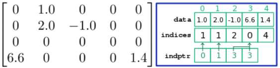
The array denoted data stores the values of the non-zero elements of the matrix, in sequential order from left to right along each row, then from the top row to the bottom. The array denoted indices records the column index for each of these elements. In the above example, data[3] stores a value of \(6.6\), and indices[3] has a value of \(0\), indicating that a matrix element with value \(6.6\) occurs in column \(0\). These two arrays have the same length, equal to the number of non-zero elements in the sparse matrix.

The array denoted indptr (which stands for "index pointer") provides an association between the row indices and the matrix elements, but in an indirect manner. Its length is equal to the number of matrix rows (including zero rows). For each row \(i\), if the row is non-zero, indptr[i] records the index in the data and indices arrays corresponding to the first non-zero element on row \(i\). (For a zero row, indptr records the index of the next non-zero element occurring in the matrix.)

For example, consider looking up index \((1,2)\) in the above figure. The row index is 1, so we examine indptr[1] (whose value is \(1\)) and indptr[2] (whose value is \(3\)). This means that the non-zero elements for matrix row \(1\) correspond to indices \(1 \le n < 3\) of the data and indices arrays. We search indices[1] and indices[2], looking for a column index of \(2\). This is found in indices[2], so we look in data[2] for the value of the matrix element, which is \(-1.0\).

It is clear that looking up an individual matrix element is very efficient. Unlike the LIL format, where we need to step through a linked list, in the CSR format the indptr array lets us to jump straight to the data for the relevant row. For the same reason, the CSR format is efficient for row slicing operations (e.g., A[4,:]), and for matrix-vector products like \(\mathbf{A}\vec{x}\) (which involves taking the product of each matrix row with the vector \(\vec{x}\)).

The CSR format does have several downsides. Column slicing (e.g. A[:,4]) is inefficient, since it requires searching through all elements of the indices array for the relevant column index. Changes to the sparsity structure (e.g., inserting new elements) are also very inefficient, since all three arrays need to be re-arranged.

To create a sparse matrix in the CSR format, we use the csr_matrix function, which is provided by the scipy.sparse module. Here is an example program:

from scipy import *
import scipy.sparse as sp

data = [1.0, 2.0, -1.0, 6.6, 1.4]
rows = [0, 1, 1, 3, 3]
cols = [1, 1, 2, 0, 4]

A = sp.csr_matrix((data, [rows, cols]), shape=(4,5))
print(A)

Here, the first input to csr_matrix is a tuple of the form (data, idx), where data is a 1D array specifying the non-zero matrix elements, idx[0,:] specifies the row indices, and idx[1,:] specifies the column indices. Running the program produces the expected results:

 (0, 1)	1.0
 (1, 1)	2.0
 (1, 2)	-1.0
 (3, 0)	6.6
 (3, 4)	1.4

The csr_matrix function figures out and generates the three CSR arrays automatically; you don't need to work them out yourself. But if you like, you can inspect the contents of the CSR arrays directly:

>>> A.data
array([ 1. ,  2. , -1. ,  6.6,  1.4])
>>> A.indices
array([1, 1, 2, 0, 4], dtype=int32)
>>> A.indptr
array([0, 1, 3, 3, 5], dtype=int32)

(There is an extra trailing element of \(5\) in the indptr array. For simplicity, we didn't mention this in the above discussion, but you should be able to figure out why it's there.)

Another way to create a CSR matrix is to first create a matrix in another format (e.g. a conventional 2D array, or a sparse matrix in LIL format), and provide that as the input to csr_matrix. This returns the specified matrix in CSR format. For example:

>>> A = sp.lil_matrix((6,6))
>>> A[0,1] = 4.0
>>> A[2,0] = 5.0
>>> B = sp.csr_matrix(A)

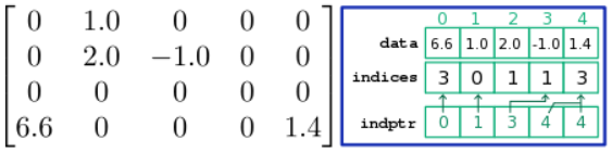
8.2.4 Compressed Sparse Column (CSC)

The Compressed Sparse Column (CSC) format is very similar to the CSR format, except that the role of rows and columns is swapped. The data array stores non-zero matrix elements in sequential order from top to bottom along each column, then from the left-most column to the right-most. The indices array stores row indices, and each element of the indptr array corresponds to one column of the matrix. An example is shown below:

Figure \(\PageIndex{4}\): A sparse matrix and its representation in Compressed Sparse Column (CSC) format.

The CSC format is efficient at matrix lookup, column slicing operations (e.g., A[:,4]), and vector-matrix products like \(\vec{x}^{\,T} \mathbf{A}\) (which involves taking the product of the vector \(\vec{x}\) with each matrix column). However, it is inefficient for row slicing (e.g. A[4,:]), and for changes to the sparsity structure.

To create a sparse matrix in the CSC format, we use the csc_matrix function. This is analogous to the csr_matrix function for CSR matrices. For example,

>>> from scipy import *
>>> import scipy.sparse as sp
>>> data = [1.0, 2.0, -1.0, 6.6, 1.4]
>>> rows = [0, 1, 1, 3, 3]
>>> cols = [1, 1, 2, 0, 4]
>>> 
>>> A = sp.csc_matrix((data, [rows, cols]), shape=(4,5))
>>> A
<4x5 sparse matrix of type '<class 'numpy.float64'>'
  with 5 stored elements in Compressed Sparse Column format>