8.4: Example- Particle-in-a-Box Problem

Last updated
Save as PDF

Page ID: 34849

\( \newcommand{\vecs}[1]{\overset { \scriptstyle \rightharpoonup} {\mathbf{#1}} } \) \( \newcommand{\vecd}[1]{\overset{-\!-\!\rightharpoonup}{\vphantom{a}\smash {#1}}} \)\(\newcommand{\id}{\mathrm{id}}\) \( \newcommand{\Span}{\mathrm{span}}\) \( \newcommand{\kernel}{\mathrm{null}\,}\) \( \newcommand{\range}{\mathrm{range}\,}\) \( \newcommand{\RealPart}{\mathrm{Re}}\) \( \newcommand{\ImaginaryPart}{\mathrm{Im}}\) \( \newcommand{\Argument}{\mathrm{Arg}}\) \( \newcommand{\norm}[1]{\| #1 \|}\) \( \newcommand{\inner}[2]{\langle #1, #2 \rangle}\) \( \newcommand{\Span}{\mathrm{span}}\) \(\newcommand{\id}{\mathrm{id}}\) \( \newcommand{\Span}{\mathrm{span}}\) \( \newcommand{\kernel}{\mathrm{null}\,}\) \( \newcommand{\range}{\mathrm{range}\,}\) \( \newcommand{\RealPart}{\mathrm{Re}}\) \( \newcommand{\ImaginaryPart}{\mathrm{Im}}\) \( \newcommand{\Argument}{\mathrm{Arg}}\) \( \newcommand{\norm}[1]{\| #1 \|}\) \( \newcommand{\inner}[2]{\langle #1, #2 \rangle}\) \( \newcommand{\Span}{\mathrm{span}}\)

To demonstrate the use of sparse matrices for solving finite-difference equations, we consider the 1D particle-in-a-box problem. This consists of the 1D time-independent Schrödinger wave equation,

\[-\frac{1}{2} \, \frac{d^2\psi}{dx^2} = E\psi(x), \quad 0 \le x \le L,\]

together with the Dirichlet boundary conditions

\[\psi(0) = \psi(L) = 0.\]

The analytic solution is well known to us; up to a normalization factor, the eigenstates and energy eigenvalues are

\[\psi_m(x) = \sin\Big(m\pi x / L\Big),\quad E_m = \frac{1}{2}\, \left(\frac{m\pi}{L}\right)^2, \quad m = 1, 2, 3, \dots\]

We will write a program that seeks a numerical solution. Using the three-point rule to discretize the second derivative, the finite-difference matrix equations become

\[-\frac{1}{2h^2}\begin{bmatrix} -2 & 1 \\ 1 & -2 & \ddots \\ & \ddots & \ddots & 1 \\ & & 1 & -2\end{bmatrix} \begin{bmatrix}\psi_0 \\ \psi_1 \\ \vdots \\ \psi_{N-1}\end{bmatrix} = E \begin{bmatrix}\psi_0 \\ \psi_1 \\ \vdots \\ \psi_{N-1}\end{bmatrix},\]

where

\[h = \frac{L}{N + 1}, \quad \psi_n = \psi\Big(x = h(n+1)\Big)\]

The following program constructs the finite-difference matrix equation, and displays the first three solutions:

from scipy import *
import scipy.sparse as sp
import scipy.sparse.linalg as spl
import matplotlib.pyplot as plt

## Solve the 1D particle-in-a-box problem for box length L,
## using N discretization points.  The parameter nev is the
## number of eigenvalues/eigenvectors to find.  Return three
## arrays E, psi, and x.  E stores the energy eigenvalues;
## psi stores the (non-normalized) eigenstates; and x stores
## the discretization points.
def particle_in_a_box(L, N, nev=3):
    dx = L/(N+1.0)
    x  = linspace(dx, L-dx, N)
    I  = ones(N)
    ## Set up the finite-difference matrix.
    H  = sp.dia_matrix(([I, -2*I, I], [-1,0,1]), shape=(N,N))
    H *= -0.5/(dx*dx)
    ## Find the lowest eigenvalues and eigenvectors.
    E, psi = spl.eigsh(H, k=nev, sigma=-1.0)
    return E, psi, x

def particle_in_a_box_demo():
    E, psi, x = particle_in_a_box(1.0, 1000)

    ## Print the energy eigenvalues.
    print(E)

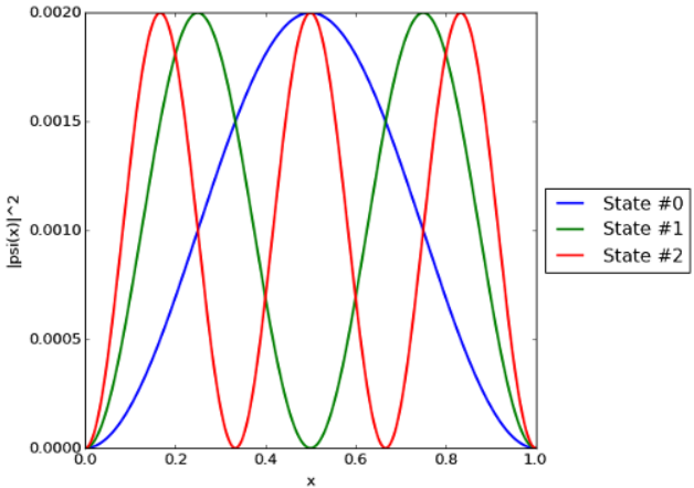
    ## Plot |psi(x)|^2 vs x for each solution found.
    fig = plt.figure()
    axs = plt.subplot(1,1,1)
    for n in range(len(E)):
        fig_label = "State #" + str(n)
        plt.plot(x, abs(psi[:,n])**2, label=fig_label, linewidth=2)
    plt.xlabel('x')
    plt.ylabel('|psi(x)|^2')

    ## Shrink the axis by 20%, so the legend can fit.
    box = axs.get_position()
    axs.set_position([box.x0, box.y0, box.width * 0.8, box.height])
    ## Print the legend.
    plt.legend(loc='center left', bbox_to_anchor=(1, 0.5))
    plt.show()

particle_in_a_box_demo()

The Hamiltonian matrix, which is tridiagonal, is constructed in the DIA sparse matrix format. The eigenvalues and eigenvectors are found with eigsh, which can be used because the Hamiltonian matrix is known to be Hermitian. Notice that we call eigsh using the sigma parameter, telling the eigensolver to find the eigenvalues closest in value to \(-1.0\):

    E, psi = spl.eigsh(H, k=nev, sigma=-1.0)

This will find the lowest energy eigenvalues because, in this case, all energy eigenvalues are positive. (We use \(-1.0\) instead of 0.0, because the algorithm does not work well when sigma is exactly zero.) If there is a negative potential present, we would have to find a different estimate for the lower bound of the energy eigenvalues, and pass that to sigma.

Alternatively, we could have called eigsh with an input which='SA'. This would tell the eigensolver to find the eigenvalue with the smallest value. We avoid doing this because the ARPACK eigensolver algorithm is relatively inefficient at finding small eigenvalues in which mode (and it can sometimes even fail to converge, if k is too small). Typically, if you are able to deduce a lower bound for the desired eigenvalues, it is preferable to use sigma.

Running the program prints the lowest energy eigenvalues:

[  4.93479815  19.73914399  44.41289171]

This agrees well with the analytical results \(E_1 = \pi^2/2 = 4.934802\), \(E_2 = 2\pi^2 = 19.739208\), and \(E_3=9\pi^2/2 = 44.413219\). It also produces the plot shown below, which is likewise as expected.

Figure \(\PageIndex{1}\): Plots of \(|\psi(x)|^2\) versus \(x\) for the particle-in-a-box problem.