5.2: The Deuteron

Reduced Hamiltonian in the center-of-mass frame

We start with the simplest problem, a nucleus formed by just one neutron and one proton: the deuteron. We will at first neglect the spins of these two particles and solve the energy eigenvalue problem (time-independent Schrödinger equation) for a bound p-n system. The Hamiltonian is then given by the kinetic energy of the proton and the neutron and by their mutual interaction.

\[\mathcal{H}=\frac{1}{2 m_{n}} \hat{p}_{n}^{2}+\frac{1}{2 m_{p}} \hat{p}_{p}^{2}+V_{n u c}\left(\left|x_{p}-x_{n}\right|\right) \nonumber\]

Here we stated that the interaction depends only on the distance between the two particles (and not for example the angle...)

We could try to solve the Schrödinger equation for the wavefunction \(\Psi=\Psi\left(\vec{x}_{p}, \vec{x}_{n}, t\right) \). This is a wavefunction that treats the two particles as fundamentally independent (that is, described by independent variables). However, since the two particles are interacting, it might be better to consider them as one single system. Then we can use a different type of variables (position and momentum).

We can make the transformation from \(\left\{\vec{x}_{p}, \vec{x}_{n}\right\} \rightarrow\{\vec{R}, \vec{r}\}\) where \(\vec{R}\) describes the average position of the two particles (i.e. the position of the total system, to be accurately defined) and \( \vec{r}\) describes the relative position of one particle wrt the other:

\[\left\{\begin{array}{ll}
\vec{R}=\frac{m_{p} \vec{x}_{p}+m_{n} \vec{x}_{n}}{m_{p}+m_{n}} & \text { center of mass } \\
\vec{r}=\vec{x}_{p}-\vec{x}_{n} & \text { relative position }
\end{array}\right. \nonumber\]

We can also invert these equations and define \(\vec{x}_{p}=x_{p}(\vec{R}, \vec{r})\) and \(\vec{x}_{n}=x_{n}(\vec{R}, \vec{r})\). Also, we can define the center of mass momentum and relative momentum (and velocity):

\[\left\{\begin{array}{l}
\vec{p}_{c m}=\vec{p}_{p}+\vec{p}_{n} \\
\vec{p}_{r}=\left(m_{n} \vec{p}_{p}-m_{p} \vec{p}_{n}\right) / M
\end{array}\right. \nonumber\]

Then the (classical) Hamiltonian, using these variables, reads

\[H=\frac{1}{2 M} p_{c m}^{2}+\frac{1}{2 \mu} p_{r}^{2}+V_{n u c}(|r|) \nonumber\]

where \( M=m_{p}+m_{n}\) and \(\mu=\frac{m_{p} m_{n}}{m_{p}+m_{n}} \) is the reduced mass. Now we can just write the quantum version of this classical Hamiltonian, using

\[\hat{p}_{c m}=-i \hbar \frac{\partial}{\partial \vec{R}} \quad \hat{p}_{r}=-i \hbar \frac{\partial}{\partial \vec{r}} \nonumber\]

in the equation

\[\mathcal{H}=\frac{1}{2 M} \hat{p}_{c m}^{2}+\frac{1}{2 \mu} \hat{p}_{r}^{2}+V_{n u c}(|\hat{r}|) \nonumber\]

Now, since the variables r and R are independent (same as \( r_{p}\) and \( r_{n}\)) they commute. This is also true for \( p_{c m}\) and r (and \( p_{r}\) and R). Then, \( p_{c m}\) commutes with the whole Hamiltonian, \( \left[\hat{\vec{p}}_{c m}, \mathcal{H}\right]=0\). This implies that \( \hat{\vec{p}}_{c m}\) is a constant of the motion. This is also true for \( E_{c m}=\frac{1}{2 M} \hat{\vec{p}}_{c m}^{2}\), the energy of the center of mass. If we solve the problem in the center-of-mass frame, then we can set \(E_{c m}=0 \) and this is not ever going to change. In general, it means that we can ignore the first term in the Hamiltonian and just solve

\[\mathcal{H}_{D}=-\frac{\hbar^{2}}{2 \mu} \nabla_{r}^{2}+V_{n u c}(|\vec{r}|) \nonumber\]

In practice, this corresponds to having applied separation of variables to the original total Schrödinger equation. The Hamiltonian \(\mathcal{H}_{D} \) (the deuteron Hamiltonian) is now the Hamiltonian of a single-particle system, describing the motion of a reduced mass particle in a central potential (a potential that only depends on the distance from the origin). This motion is the motion of a neutron and a proton relative to each other. In order to proceed further we need to know the shape of the central potential.

Ground state

What are the most important characteristics of the nuclear potential? It is known to be very strong and short range. These are the only characteristics that are of interest now; also, if we limit ourselves to these characteristics and build a simple, fictitious potential based on those, we can hope to be able to solve exactly the problem.

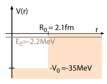
If we looked at a more complex, albeit more realistic, potential, then most probably we cannot find an exact solution and would have to simplify the problem. Thus, we just take a very simple potential, a nuclear square well of range \(R_{0} \approx 2.1 f m\) and of depth \(-V_{0}=-35 \ \mathrm{MeV}\).

We need to write the Hamiltonian in spherical coordinates (for the reduced variables). The kinetic energy term is given by:

\[-\frac{\hbar^{2}}{2 \mu} \nabla_{r}^{2}=-\frac{\hbar^{2}}{2 \mu} \frac{1}{r^{2}} \frac{\partial}{\partial r}\left(r^{2} \frac{\partial}{\partial r}\right)-\frac{\hbar^{2}}{2 \mu r^{2}}\left[\frac{1}{\sin \vartheta} \frac{\partial}{\partial \vartheta}\left(\sin \vartheta \frac{\partial}{\partial \vartheta}\right)+\frac{1}{\sin ^{2} \vartheta} \frac{\partial^{2}}{\partial \varphi^{2}}\right]=-\frac{\hbar^{2}}{2 \mu} \frac{1}{r^{2}} \frac{\partial}{\partial r}\left(r^{2} \frac{\partial}{\partial r}\right)+\frac{\hat{L}^{2}}{2 \mu r^{2}} \nonumber \]

Figure \(\PageIndex{1}\): Nuclear potential (CC BY-NC-ND; Paola Cappellaro)

where we used the angular momentum operator (for the reduced particle) \(\hat{L}^{2}\).

The Schrödinger equation then reads

\[\left[-\frac{\hbar^{2}}{2 \mu} \frac{1}{r^{2}} \frac{\partial}{\partial r}\left(r^{2} \frac{\partial}{\partial r}\right)+\frac{\hat{L}^{2}}{2 \mu r^{2}}+V_{n u c}(r)\right] \Psi_{n, l, m}(r, \vartheta, \varphi)=E_{n} \Psi_{n, l, m}(r, \vartheta, \varphi) \nonumber\]

We can now also check that \(\left[\hat{L}^{2}, \mathcal{H}\right]=0\). Then \(\hat{L}^{2}\) is a constant of the motion and it has common eigenfunctions with the Hamiltonian.

We have already solved the eigenvalue problem for the angular momentum. We know that solutions are the spherical harmonics \(Y_{l}^{m}(\vartheta, \varphi)\):

\[\hat{L}^{2} Y_{l}^{m}(\vartheta, \varphi)=\hbar^{2} l(l+1) Y_{l}^{m}(\vartheta, \varphi) \nonumber\]

Then we can solve the Hamiltonian above with the separation of variables methods, or more simply look for a solution \(\Psi_{n, l, m}=\psi_{n, l}(r) Y_{l}^{m}(\vartheta, \varphi)\):

\[-\frac{\hbar^{2}}{2 \mu} \frac{1}{r^{2}} \frac{\partial}{\partial r}\left(r^{2} \frac{\partial \psi_{n, l}(r)}{\partial r}\right) Y_{l}^{m}(\vartheta, \varphi)+\psi_{n, l}(r) \frac{\hat{L}^{2}\left[Y_{l}^{m}(\vartheta, \varphi)\right]}{2 \mu r^{2}}=\left[E_{n}-V_{n u c}(r)\right] \psi_{n, l}(r) Y_{l}^{m}(\vartheta, \varphi) \nonumber\]

and then we can eliminate \( Y_{l}^{m}\) to obtain:

\[-\frac{\hbar^{2}}{2 \mu} \frac{1}{r^{2}} \frac{d}{d r}\left(r^{2} \frac{d \psi_{n, l}(r)}{d r}\right)+\left[V_{n u c}(r)+\frac{\hbar^{2} l(l+1)}{2 \mu r^{2}}\right] \psi_{n, l}(r)=E_{n} \psi_{n, l}(r) \nonumber\]

Now we write \( \psi_{n, l}(r)=u_{n, l}(r) / r\). Then the radial part of the Schrödinger equation becomes

\[-\frac{\hbar^{2}}{2 \mu} \frac{d^{2} u}{d r^{2}}+\left[V_{n u c}(r)+\frac{\hbar^{2}}{2 \mu} \frac{l(l+1)}{r^{2}}\right] u(r)=E u(r) \nonumber\]

with boundary conditions

\[\begin{array}{l}
u_{n l}(0)=0 \quad \rightarrow \quad \psi(0) \text { is finite } \\
u_{n l}(\infty)=0 \quad \rightarrow \quad \text { bound state }
\end{array} \nonumber\]

This equation is just a 1D Schrödinger equation in which the potential \(V(r)\) is replaced by an effective potential

\[V_{e f f}(r)=V_{n u c}(r)+\frac{\hbar^{2} l(l+1)}{2 \mu r^{2}} \nonumber\]

that presents the addition of a centrifugal potential (that causes an outward force).

Figure \(\PageIndex{2}\): Nuclear potential for \( l \neq 0\). Left, nuclear potential and centrifugal potential. Right, the effective potential (CC BY-NC-ND; Paola Cappellaro)

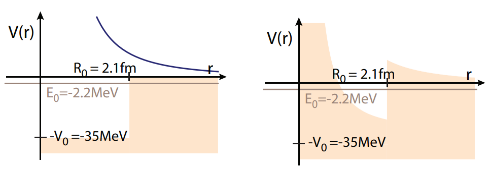
Notice that if \(l\) is large, the centrifugal potential is higher. The ground state is then found for \(l\) = 0. In that case there is no centrifugal potential and we only have a square well potential (that we already solved).

\[\left[-\frac{\hbar^{2}}{2 \mu} \frac{1}{r} \frac{\partial^{2}}{\partial r}+V_{n u c}(r)\right] u_{0}(r)=E_{0} u_{0}(r) \nonumber\]

This gives the eigenfunctions

\[u(r)=A \sin (k r)+B \cos (k r), \quad 0<r<R_{0} \nonumber\]

and

\[u(r)=C e^{-\kappa r}+D e^{\kappa r}, \quad r>R_{0} \nonumber\]

The allowed eigenfunctions (as determined by the boundary conditions) have eigenvalues found from the odd-parity solutions to the equation

\[-\kappa=k \cot \left(k R_{0}\right) \nonumber\]

with

\[k^{2}=\frac{2 \mu}{\hbar^{2}}\left(E_{0}+V_{0}\right) \quad \kappa^{2}=-\frac{2 \mu}{\hbar^{2}} E_{0} \nonumber\]

(with \(E_{0}<0\)).

Recall that we found that there was a minimum well depth and range in order to have a bound state. To satisfy the continuity condition at \(r=R_{0}\) we need \(\lambda / 4 \leq R_{0}\) or \(k R_{0} \geq \frac{1}{4} 2 \pi=\frac{\pi}{2}\). Then \(R_{0} \geq \frac{\pi}{2 k}\).

In order to find a bound state, we need the potential energy to be higher than the kinetic energy \(V_{0}>E_{k i n}\). If we know \(R_{0}\) we can use \(k \geq \frac{\pi}{2 R_{0}}\) to find

\[V_{0}>\frac{\hbar^{2} \pi^{2}}{2 \mu 4 R_{0}^{2}}=\frac{\pi^{2}}{8} \frac{\hbar^{2} c^{2}}{\mu c^{2} R_{0}^{2}}=\frac{\pi^{2}}{8} \frac{(191 M e V f m)^{2}}{469 M e V(2.1 f m)^{2}}=23.1 M e V \nonumber\]

We thus find that indeed a bound state is possible, but the binding energy \(E_{0}=E_{k i n}-V_{0}\) is quite small. Solving numerically the trascendental equation for E₀ we find that

\[\boxed{E_{0}=-2.2 \mathrm{MeV}} \nonumber\]

Notice that in our procedure we started from a model of the potential that includes the range \(R_{0} \) and the strength \(V_{0} \) in order to find the ground state energy (or binding energy). Experimentally instead we have to perform the inverse process. From scattering experiments it is possible to determine the binding energy (such that the neutron and proton get separated) and from that, based on our theoretical model, a value of \( V_{0}\) can be inferred.

Deuteron excited state

Are bound excited states for the deuteron possible?

Consider first \(l\) = 0. We saw that the binding energy for the ground state was already small. The next odd solution would have \(k=\frac{3 \pi}{2 R_{0}}=3 k_{0}\). Then the kinetic energy is 9 times the ground state kinetic energy or \(E_{k i n}^{1}=9 E_{k i n}^{0}=9 \times 32.8 M e V=295.2 M e V . \). The total energy thus becomes positive, the indication that the state is no longer bound (in fact, we then have no longer a discrete set of solutions, but a continuum of solutions).

Consider then \(l\) > 0. In this case the potential is increased by an amount \(\frac{\hbar^{2} l(l+1)}{2 \mu R_{0}^{2}} \geq 18.75 M e V \) (for \(l\) = 1). The potential thus becomes shallower (and narrower). Thus also in this case the state is no longer bound. The deuteron has only one bound state.

Spin dependence of nuclear force

Until now we neglected the fact that both neutron and proton possess a spin. The question remains how the spin influences the interaction between the two particles.

The total angular momentum for the deuteron (or in general for a nucleus) is usually denoted by I. Here it is given by

\[\hat{\vec{I}}=\hat{\vec{L}}+\hat{\vec{S}}_{p}+\hat{\vec{S}}_{n} \nonumber\]

For the bound deuteron state \(l\) = 0 and \(\hat{\vec{I}}=\hat{\vec{S}}_{p}+\hat{\vec{S}}_{n}=\hat{\vec{S}}\). A priori we can have \(\hat{\vec{S}}=0\) or 1 (recall the rules for addition of angular momentum, here \(\hat{\vec{S}}_{p, n}=\frac{1}{2}\)).

There are experimental signatures that the nuclear force depends on the spin. In fact the deuteron is only found with \(\hat{\vec{S}}=1\) (meaning that this configuration has a lower energy).

The simplest form that a spin-dependent potential could assume is \( V_{\text {spin}} \propto \hat{\vec{S}}_{p} \cdot \hat{\vec{S}}_{n}\) (since we want the potential to be a scalar). The coefficient of proportionality \(V_{1}(r) / \hbar^{2}\) can have a spatial dependence. Then, we guess the form for the spin-dependent potential to be \(V_{s p i n}=V_{1}(r) / \hbar^{2} \hat{\vec{S}}_{p} \cdot \hat{\vec{S}}_{n}\). What is the potential for the two possible configurations of the neutron and proton spins?

The configuration are either \(\hat{\vec{S}}=1\) or \(\hat{\vec{S}}=0\). Let us write \(\hat{\vec{S}}^{2}=\hbar S(S+1)\) in terms of the two spins:

\[\hat{\vec{S}}^{2}=\hat{\vec{S}}_{p}^{2}+\hat{\vec{S}}_{n}^{2}+2 \hat{\vec{S}}_{p} \cdot \hat{\vec{S}}_{n} \nonumber\]

The last term is the one we are looking for:

\[\hat{\vec{S}}_{p} \cdot \hat{\vec{S}}_{n}=\frac{1}{2}\left(\hat{\vec{S}}^{2}-\hat{\vec{S}}_{p}^{2}-\hat{\vec{S}}_{n}^{2}\right) \nonumber\]

Because \(\hat{S}^{2} \) and \( \hat{\vec{S}}_{p}^{2}, \hat{\vec{S}}_{n}^{2}\) commute, we can write an equation for the expectation values wrt eigenfunctions of these operators¹⁰:

\[\left\langle\hat{\vec{S}}_{p} \cdot \hat{\vec{S}}_{n}\right\rangle=\left\langle S, S_{p}, S_{n}, S_{z}\left|\hat{\vec{S}}_{p} \cdot \hat{\vec{S}}_{n}\right| S, S_{p}, S_{n}, S_{z}\right\rangle=\frac{\hbar^{2}}{2}\left(S(S+1)-S_{p}\left(S_{p}+1\right)-S_{n}\left(S_{n}+1\right)\right) \nonumber\]

since \( S_{p, n}=\frac{1}{2}\), we obtain

\[\left\langle\hat{\vec{S}}_{p} \cdot \hat{\vec{S}}_{n}\right\rangle=\frac{\hbar^{2}}{2}\left(S(S+1)-\frac{3}{2}\right)=\begin{array}{ll}
+\frac{\hbar^{2}}{4} & \text { Triplet State, }\left|S=1, \frac{1}{2} \frac{1}{2}, m_{z}\right\rangle \\
-\frac{3 \hbar^{2}}{4} & \text { singlet State, }\left|S=0, \frac{1}{2}, \frac{1}{2}, 0\right\rangle
\end{array} \nonumber\]

If V₁(r) is an attractive potential (< 0), the total potential is \(\left.V_{n u c}\right|_{S=1}=V_{T}=V_{0}+\frac{1}{4} V_{1}\) for a triplet state, while its strength is reduced to \(\left.V_{n u c}\right|_{S=0}=V_{S}=V_{0}-\frac{3}{4} V_{1}\) for a singlet state. How large is V₁?

We can compute V₀ and V₁ from knowing the binding energy of the triplet state and the energy of the unbound virtual state of the singlet (since this is very close to zero, it can still be obtained experimentally). We have \(E_{T}=-2.2 \mathrm{MeV}\) (as before, since this is the experimental data) and \( E_{S}=77 \mathrm{keV}\). Solving the eigenvalue problem for a square well, knowing the binding energy E_T and setting E_S ≈ 0, we obtain V_T = −35MeV and V_S = −25MeV (Notice that of course V_T is equal to the value we had previously set for the deuteron potential in order to find the correct binding energy of 2.2MeV, we just –wrongly– neglected the spin earlier on). From these values by solving a system of two equations in two variables:

\[\left\{\begin{array}{l}
V_{0}+\frac{1}{4} V_{1}=V_{T} \\
V_{0}-\frac{3}{4} V_{1}=V_{S}
\end{array}\right. \nonumber\]

we obtain V₀ = −32.5MeV V₁ = −10MeV. Thus the spin-dependent part of the potential is weaker, but not negligible.

Note

10 Note that of course we use the coupled representation since the properties of the deuteron, and of its spin-dependent energy, are set by the common state of proton and neutron