5.3: Nuclear Models

In the case of the simplest nucleus (the deuterium, with 1p-1n) we have been able to solve the time independent Schrödinger equation from first principles and find the wavefunction and energy levels of the system —of course with some approximations, simplifying for example the potential. If we try to do the same for larger nuclei, we soon would find some problems, as the number of variables describing position and momentum increases quickly and the math problems become very complex.

Another difficulty stems from the fact that the exact nature of the nuclear force is not known, as there’s for example some evidence that there exist also 3-body interactions, which have no classical analog and are difficult to study via scattering experiments.

Then, instead of trying to solve the problem exactly, starting from a microscopic description of the nucleus constituents, nuclear scientists developed some models describing the nucleus. These models need to yield results that agree with the already known nuclear properties and be able to predict new properties that can be measured in experiments. We are now going to review some of these models.

Shell structure

The atomic shell model

You might already be familiar with the atomic shell model. In the atomic shell model, shells are defined based on the atomic quantum numbers that can be calculated from the atomic Coulomb potential (and ensuing the eigenvalue equation) as given by the nuclear’s protons.

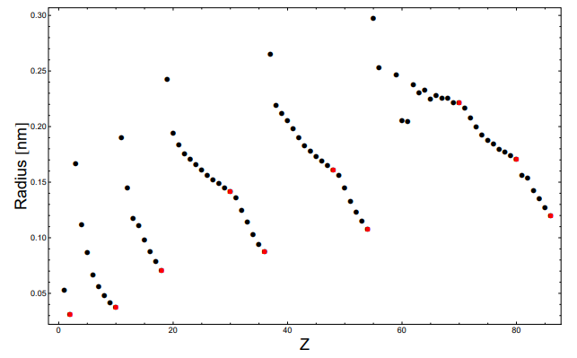
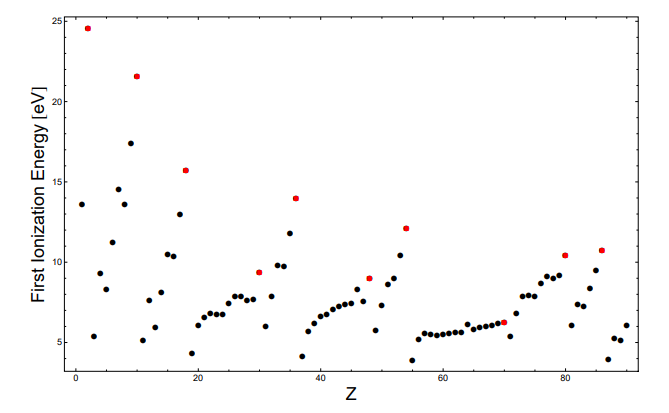
Shells are filled by electrons in order of increasing energies, such that each orbital (level) can contain at most 2 electrons (by the Pauli exclusion principle). The properties of atoms are then mostly determined by electrons in a non-completely filled shell. This leads to a periodicity of atomic properties, such as the atomic radius and the ionization energy, that is reflected in the periodic table of the elements. We have seen when solving for the hydrogen

Figure $\PageIndex{1}$: Atomic Radius vs Z. (CC BY-NC-ND; Paola Cappellaro)

atom that a quantum state is described by the quantum numbers: $|\psi=| n, l, m$ where $n$ is the principle quantum number (that in the hydrogen atom was giving the energy). $l$ is the angular momentum quantum number (or azimuthal quantum number ) and $m$ the magnetic quantum number. This last one is $m=-l, \ldots, l-1, l$ thus together with the spin quantum number, sets the degeneracy of each orbital (determined by $n$ and $l < n$) to be $D(l) = 2(2l + 1)$. Historically, the orbitals have been called with the spectroscopic notation as follows:

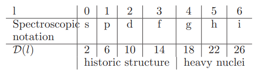
The historical notations come from the description of the observed spectral lines:

$$\mathbf{s}=\operatorname{sharp} \quad \mathbf{p}=\text { principal } \quad \mathbf{d}=\text { diffuse } \quad \mathbf{f}=\text { fine } \nonumber$$

Figure $\PageIndex{2}$: Ionization energy vs Z. (CC BY-NC-ND; Paola Cappellaro)

Orbitals (or energy eigenfunctions) are then collected into groups of similar energies (and similar properties). The degeneracy of each orbital gives the following (cumulative) occupancy numbers for each one of the energy group:

$$\boxed{\begin{array}{lllll} 2, & 10, & 18, & 36, & 54, & 70, & 86 \end{array}} \nonumber$$

Notice that these correspond to the well known groups in the periodic table.

There are some difficulties that arise when trying to adapt this model to the nucleus, in particular the fact that the potential is not external to the particles, but created by themselves, and the fact that the size of the nucleons is much larger than the electrons, so that it makes much less sense to speak of orbitals. Also, instead of having just one type of particle (the electron) obeying Pauli’s exclusion principle, here matters are complicated because we need to fill shells with two types of particles, neutrons and protons.

In any case, there are some compelling experimental evidences that point in the direction of a shell model.

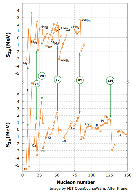
Evidence of nuclear shell structure: Two-nucleon separation energy

The two-nucleon separation energy (2p- or 2n-separation energy) is the equivalent of the ionization energy for atoms, where nucleons are taken out in pair to account for a term in the nuclear potential that favor the pairing of nucleons. From this first set of data we can infer that there exist shells with occupation numbers

$$\boxed{\begin{array}{lllll} 8, & 20, & 28, & 50, & 82, & 126\end{array}} \nonumber$$

These are called Magic numbers in nuclear physics. Comparing to the size of the atomic shells, we can see that the atomic magic numbers are quite different from the nuclear ones (as expected since there are two-types of particles and other differences.) Only the guiding principle is the same. The atomic shells are determined by solving the energy eigenvalue equation. We can attempt to do the same for the nucleons.

Nucleons Hamiltonian

The Hamiltonian for the nucleus is a complex many-body Hamiltonian. The potential is the combination of the nuclear and coulomb interaction:

$$\mathcal{H}=\sum_{i} \frac{\hat{p}_{i}^{2}}{2 m_{i}}+\sum_{j, i \leq j} V_{n u c}\left(\left|\vec{x}_{i}-\vec{x}_{j}\right|\right)+\underbrace{\sum_{j, i \leq j} \frac{e^{2}}{\left|\vec{x}_{i}-\vec{x}_{j}\right|}}_{\text {sum on protons only }} \nonumber$$

There is not an external potential as for the electrons (where the protons create a strong external central potential for each electron). We can still simplify this Hamiltonian by using mean field theory¹¹.

Note

11 This is a concept that is relevant in many other physical situations

Figure $\PageIndex{3}$: Top: Two-proton separation energies of isotones (constant N). Bottom: two-neutron separation energies of isotopes (constant Z). On the x-axis: nucleon number. The sudden changes at the magic number are apparent. From Krane, fig 5.2

We can rewrite the Hamiltonian above by picking 1 nucleon, e.g. the $j^{t h}$ neutron:

$$\mathcal{H}_{j}^{n}=\frac{\hat{p}_{j}^{2}}{2 m_{n}}+\sum_{i \leq j} V_{n u c}\left(\left|\vec{x}_{i}-\vec{x}_{j}\right|\right) \nonumber$$

or the $k^{t h}$ proton:

$$\mathcal{H}_{k}^{p}=\frac{\hat{p}_{k}^{2}}{2 m_{n}}+\sum_{i \leq k} V_{n u c}\left(\left|\vec{x}_{i}-\vec{x}_{k}\right|\right)+\underbrace{\sum_{i \leq k} \frac{e^{2}}{\left|\vec{x}_{i}-\vec{x}_{k}\right|}}_{\text {sum on protons only }} \nonumber$$

then the total Hamiltonian is just the sum over these one-particle Hamiltonians:

$$\mathcal{H}=\sum_{j \text { (neutrons) }} \mathcal{H}_{j}^{n}+\sum_{k(\text { protons })} \mathcal{H}_{k}^{p} \nonumber$$

The Hamiltonians $\mathcal{H}_{j}^{n}$ and $\mathcal{H}_{j}^{p}$ describe a single nucleon subjected to a potential $V_{n u c}^{j}\left(\left|\vec{x}_{j}\right|\right)$ — or $V^{j}\left(\left|\vec{x}_{j}\right|\right)=V_{n u c}^{j}\left(\left|\vec{x}_{j}\right|\right)+V_{c o u l}^{j}\left(\left|\vec{x}_{j}\right|\right)$ for a proton. These potentials are the effect of all the other nucleons on the nucleon we picked, and only their sum comes into play. The nucleon we focused on is then evolving in the mean field created by all the other nucleons. Of course this is a simplification, because the field created by the other nucleons depends also on the $j^{t h}$ nucleon, since this nucleon influences (for example) the position of the other nucleons. This kind of back-action is ignored in the mean-field approximation, and we considered the mean-field potential as fixed (that is, given by nucleons with a fixed position).

We then want to adopt a model for the mean-field $V_{n u c}^{j}$ and $V_{\text {coul}}^{j}$. Let’s start with the nuclear potential. We modeled the interaction between two nucleons by a square well, with depth −V₀ and range R₀. The range of the nuclear well is related to the nuclear radius, which is known to depend on the nuclear mass number A, as $R \sim 1.25 A^{1 / 3} \mathrm{fm}$. Then $V_{n u c}^{j}$ is the sum of many of these square wells, each with a different range (depending on the separation of the nucleons). The depth is instead almost constant at V₀ = 50MeV, when we consider large-A nuclei (this correspond to

Figure $\PageIndex{4}$: Potential obtained from the sum of many rectangular potential wells. Black, the potential range increases proportionally to the number of nucleons considered. Red, $R \sim A^{1 / 3}$. Blue, harmonic potential, that approximates the desired potential. (CC BY-NC-ND; Paola Cappellaro)

the average strength of the total nucleon potential). What is the sum of many square wells? The potential smooths out. We can approximate this with a parabolic potential. [Notice that for any continuous function, a minimum can always be approximated by a parabolic function, since a minimum is such that the first derivative is zero]. This type of potential is useful because we can find an analytical solution that will give us a classification of nuclear states. Of course, this is a crude approximation. This is the oscillator potential model:

$$V_{n u c} \approx-V_{0}\left(1-\frac{r^{2}}{R_{0}^{2}}\right) \nonumber$$

Now we need to consider the Coulomb potential for protons. The potential is given by: $V_{\text {coul}}=\frac{(Z-1) e^{2}}{R_{0}}\left[\frac{3}{2}-\frac{r^{2}}{2 R_{0}^{2}}\right]$ for $r \leq R_{0}$, which is just the potential for a sphere of radius R₀ containing a uniform charge $(Z-1) e$. Then we can write an effective (mean-field, in the parabolic approximation) potential as

$$V_{\mathrm{eff}}=\underbrace{r^{2}\left(\frac{V_{0}}{R_{0}^{2}}-\frac{(Z-1) e^{2}}{2 R_{0}^{3}}\right)}_{\equiv \frac{1}{2} m \omega^{2} r^{2}} \underbrace{-V_{0}+\frac{3}{2} \frac{(Z-1) e^{2}}{R_{0}}}_{\equiv-V_{0}^{\prime}} \nonumber$$

We defined here a modified nuclear square well potential $V_{0}^{\prime}=V_{0} \quad \frac{3}{2} \frac{(Z-1) e^{2}}{R_{0}}$ for protons, which is shallower than for neutrons. Also, we defined the harmonic oscillator frequencies $\omega^{2}=\frac{2}{m}\left(\frac{V_{0}}{R_{0}^{2}}-\frac{(Z-1) e^{2}}{2 R_{0}^{3}}\right)$.

The proton well is thus slightly shallower and wider than the neutron well because of the Coulomb repulsion. This potential model has limitations but it does predict the lower magic numbers.

The eigenvalues of the potential are given by the sum of the harmonic potential in 3D (as seen in recitation) and the square well:

$$E_{N}=\hbar \omega\left(N+\frac{3}{2}\right)-V_{0}^{\prime}. \nonumber$$

(where we take V₀′ = V₀ for the neutron).

Note that solving the equation for the harmonic oscillator potential is not equivalent to solve the full radial equation, where the centrifugal term $\hbar^{2} \frac{l(l+1)}{2 m r^{2}}$ must be taken into account. We could have solved that total equation and found the energy eigenvalues labeled by the radial and orbital quantum numbers. Comparing the two solutions, we find that the h.o. quantum number N can be expressed in terms of the radial and orbital quantum numbers as

$$N=2(n-1)+l \nonumber$$

Since $l=0,1, \ldots n-1$ we have the selection rule for $l$ as a function of $N: l=N, N-2, \ldots$ (with $l \geq 0$). The degeneracy of the E_N eigenvalues is then $\mathcal{D}^{\prime}(N)=\sum_{l=N, N-2, \ldots}(2 l+1)=\frac{1}{2}(N+1)(N+2)$ (ignoring spin) or $\mathcal{D}(N)=(N+1)(N+2)$ when including the spin.

We can now use these quantum numbers to fill the nuclear levels. Notice that we have separate levels for neutrons and protons. Then we can build a table of the levels occupations numbers, which predicts the first 3 magic numbers.

$$\begin{array}{|c|c|l|c|c|l|} \hline \mathrm{N} & l & \begin{array}{l} \text { Spectroscopic } \\ \text { Notation } \end{array} & \frac{1}{2} \mathcal{D}(N) & \mathcal{D}(N) & \begin{array}{l} \text { Cumulative } \\ \text { of nucle- } \\ \text { ons# } \end{array} \\ \hline 0 & 0 & 1 \mathrm{~s} & 1 & 2 & 2 \\ \hline 1 & 1 & 1 \mathrm{p} & 3 & 6 & 8 \\ \hline 2 & 0,2 & 2 \mathrm{~s}, 1 \mathrm{~d} & 6 & 12 & 20 \\ \hline \hline 3 & 1,3 & 2 \mathrm{p}, 1 \mathrm{f} & 10 & 20 & 40 \\ \hline 4 & 0,2,4 & 3 \mathrm{~s}, 2 \mathrm{~d}, 1 \mathrm{~g} & 15 & 30 & 70 \\ \hline \end{array} \nonumber$$

For higher levels there are discrepancies thus we need a more precise model to obtain a more accurate prediction. The other problem with the oscillator model is that it predicts only 4 levels to have lower energy than the 50MeV well potential (thus only 4 bound energy levels). The separation between oscillator levels is in fact $\hbar \omega=\sqrt{\frac{2 \hbar^{2} V_{0}}{m R_{0}^{2}}-\frac{(Z-1) e^{2}}{2 R_{0}^{3}}} \approx \sqrt{\frac{2 \hbar^{2} c^{2} V_{0}}{m c^{2} R_{0}^{2}}}$. Inserting the numerical values we find $\hbar \omega=\sqrt{\frac{2(200 M e V f m)^{2} \times 50 M e V}{938 M e V\left(1.25 f m A^{1 / 3}\right)^{2}}} \approx 51.5 A^{-1 / 3}$. Then the separation between oscillator levels is on the order of 10-20MeV.

Spin orbit interaction

In order to predict the higher magic numbers, we need to take into account other interactions between the nucleons. The first interaction we analyze is the spin-orbit coupling.

The associated potential can be written as

$$\frac{1}{\hbar^{2}} V_{s o}(r) \hat{\vec{l}} \cdot \hat{\vec{s}} \nonumber$$

where $\hat{\vec{s}}$ and$\hat{\vec{l}}$ are spin and angular momentum operators for a single nucleon. This potential is to be added to the single-nucleon mean-field potential seen before. We have seen previously that in the interaction between two nucleons there was a spin component. This type of interaction motivates the form of the potential above (which again is to be taken in a mean-field picture).

We can calculate the dot product with the same trick already used:

$$\langle\hat{\vec{l}} \cdot \hat{\vec{s}}\rangle=\frac{1}{2}\left(\hat{\vec{j}}^{2}-\hat{\vec{l}}^{2}-\hat{\bar{s}}^{2}\right)=\frac{\hbar^{2}}{2}\left[j(j+1)-l(l+1)-\frac{3}{4}\right] \nonumber$$

where $\hat{\vec{j}}$ is the total angular momentum for the nucleon. Since the spin of the nucleon is $s=\frac{1}{2}$, the possible values of $j$ are $j=l \pm \frac{1}{2}$. Then $j(j+1)-l(l+1)=\left(l \pm \frac{1}{2}\right)\left(l \pm \frac{1}{2}+1\right)-l(l+1)$, and we obtain

$$\langle\hat{\vec{l}} \cdot \hat{\vec{s}}\rangle=\left\{\begin{array}{ll} l \frac{\hbar^{2}}{2} & \text { for } \mathrm{j}=\mathrm{l}+\frac{1}{2} \\ -(l+1) \frac{\hbar^{2}}{2} & \text { for } \mathrm{j}=\mathrm{l}-\frac{1}{2} \end{array}\right. \nonumber$$

and the total potential is

$$V_{n u c}(r)=\left\{\begin{array}{ll} V_{0}+V_{s o} \frac{l}{2} & \text { for } \mathrm{j}=1+\frac{1}{2} \\ V_{0}-V_{s o} \frac{t+1}{2} & \text { for } \mathrm{j}=\mathrm{l}-\frac{1}{2} \end{array}\right. \nonumber$$

Now recall that both V₀ is negative and choose also V_so negative. Then:

• when the spin is aligned with the angular momentum ($j=l+\frac{1}{2}$) the potential becomes more negative, i.e. the well is deeper and the state more tightly bound.
• when spin and angular momentum are anti-aligned the system’s energy is higher.

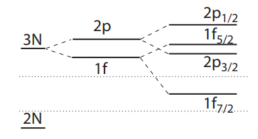
The energy levels are thus split by the spin-orbit coupling (see figure 5.3.5). This splitting is directly proportional to the angular momentum $l$ (is larger for higher $l$): $\Delta E=\frac{\hbar^{2}}{2}(2 l+1)$. The two states in the same energy configuration but with the spin aligned or anti-aligned are called a doublet.

Example $\PageIndex{1}$

Consider the N = 3 h.o. level. The level $1 f_{7 / 2}$ is pushed far down (because of the high $l$). Then its energy is so different that it makes a shell on its own. We had found that the occupation number up to N = 2 was 20 (the 3rd magic number). Then if we take the degeneracy of , , we obtain the 4th magic number 28.

[Notice that since here $j$ already includes the spin, $D(j)=2 j+1$.]

Since the $1 f_{7 / 2}$ level now forms a shell on its own and it does not belong to the N = 3 shell anymore, the residual degeneracy of N = 3 is just 12 instead of 20 as before. To this degeneracy, we might expect to have to add the lowest level of the N = 4 manifold. The highest $l$ possible for N = 4 is obtained with $n$ = 1 from the formula $N=2(n-1)+l \rightarrow l=4$ (this would be 1g). Then the lowest level is for $j=l+1 / 2=4+1 / 2=9 / 2$ with degeneracy D = 2(9/2 + 1) = 10. This new combined shell comprises then 12 + 10 levels. In turns this gives us the magic number 50.

Figure $\PageIndex{5}$: The energy levels from the harmonic oscillator level (labeled by N) are first shifted by the angular momentum potential (2p, 1f). Each l level is then split by the spin-orbit interaction, which pushes the energy up or down, depending on the spin and angular momentum alignment (CC BY-NC-ND; Paola Cappellaro)

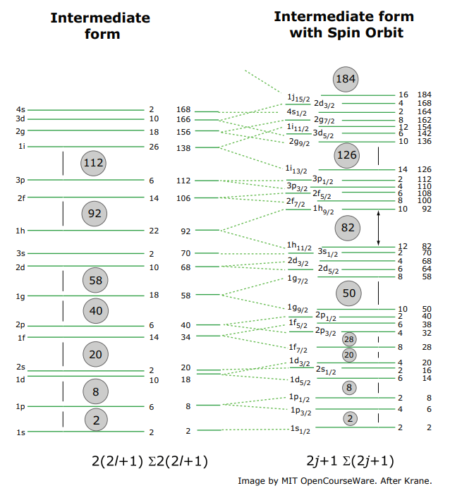
Using these same considerations, the splittings given by the spin-orbit coupling can account for all the magic numbers and even predict a new one at 184:

• N = 4, $1 \mathrm{~g} \rightarrow 1 g_{7 / 2}$ and $1 g_{9 / 2}$. Then we have 20 − 8 = 12 +D(9/2) = 10. From 28 we add another 22 to arrive at the magic number 50.
• N = 5, $1 \mathrm{~h} \rightarrow 1 h_{9 / 2}$ and $1 h_{11 / 2}$. The shell thus combines the N = 4 levels not already included above, and the $D\left(1 h_{11 / 2}\right)=12$ levels obtained from the $N=51 h_{11 / 2}$. The degeneracy of N = 4 was 30, from which we subtract the 10 levels included in N = 3. Then we have $(30-10)+D\left(1 h_{11 / 2}\right)=20+12=32$. From 50 we add arrive at the magic number 82.
• N = 6, $1 \mathrm{i} \rightarrow 1 i_{11 / 2}$ and $1 i_{13 / 2}$. The shell thus have $D(N=5)-D\left(1 h_{11 / 2}\right)+D\left(1 i_{13 / 2}\right)=42-12+14=44$ levels (D(N) = (N + 1)(N + 2)). The predicted magic number is then 126.
• $N=7 \rightarrow 1 j_{15 / 2}$ is added to the N = 6 shell, to give $D(N=6)-D\left(1 i_{13 / 2}\right)+D\left(1 j_{15 / 2}\right)=56-14+16=58$, predicting a yet not-observed 184 magic number.

Figure $\PageIndex{6}$: Shell Model prediction of the magic numbers. Level splittings due to h.o. levels, l-quantum number and spin-orbit coupling. Notice that further variations in the position of the levels are actually present (see Krane Fig. 5.6). Here only the shiftings leading to new shell groupings are shown. (CC BY-NC-ND; Paola Cappellaro)

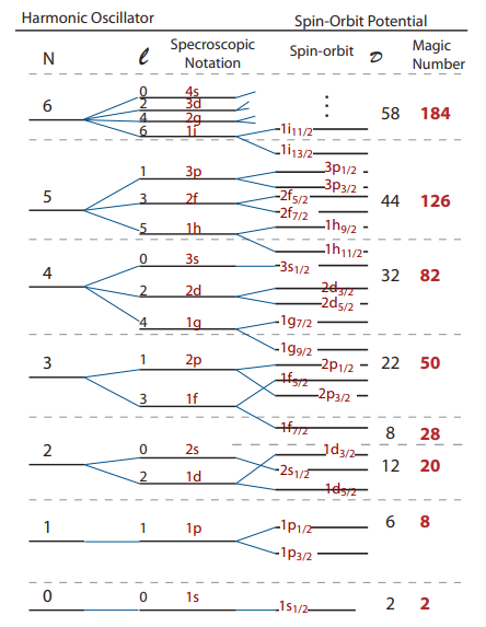
These predictions do not depend on the exact shape of the square well potential, but only on the spin-orbit coupling and its relative strength to the nuclear interaction V₀ as set in the harmonic oscillator potential (we had seen that the separation between oscillator levels was on the order of 10MeV.) In practice, if one studies in more detail the potential well, one finds that the oscillator levels with higher $l$ are lowered with respect to the others, thus enhancing the gap created by the spin-orbit coupling.

The shell model that we have just presented is quite a simplified model. However it can make many predictions about the nuclide properties. For example it predicts the nuclear spin and parity, the magnetic dipole moment and electric quadrupolar moment, and it can even be used to calculate the probability of transitions from one state to another as a result of radioactive decay or nuclear reactions.

Figure $\PageIndex{7}$: Shell Model energy levels (from Krane Fig. 5.6). Left: Calculated energy levels based on potential. To the right of each level are its capacity and cumulative number of nucleons up to that level. The spin-orbit interaction splits the levels with l > 0 into two new levels. Note that the shell effect is quite apparent, and magic numbers are reproduced exactly.

Spin pairing and valence nucleons

In the extreme shell model (or extreme independent particle model), the assumption is that only the last unpaired nucleon dictates the properties of the nucleus. A better approximation would be to consider all the nucleons above a filled shell as contributing to the properties of a nucleus. These nucleons are called the valence nucleons.

Properties that can be predicted by the characteristics of the valence nucleons include the magnetic dipole moment, the electric quadrupole moment, the excited states and the spin-parity (as we will see). The shell model can be then used not only to predict excited states, but also to calculate the rate of transitions from one state to another due to radioactive decay or nuclear reactions.

As the proton and neutron levels are filled the nucleons of each type pair off, yielding a zero angular momentum for the pair. This pairing of nucleons implies the existence of a pairing force that lowers the energy of the system when the nucleons are paired-off.

Since the nucleons get paired-off, the total spin and parity of a nucleus is only given by the last unpaired nucleon(s) (which reside(s) in the highest energy level). Specifically we can have either one neutron or one proton or a pair neutron-proton.

The parity for a single nucleon is $(-1)^{l}$, and the overall parity of a nucleus is the product of the single nucleon parity. (The parity indicates if the wavefunction changes sign when changing the sign of the coordinates. This is of course dictated by the angular part of the wavefunction – as in spherical coordinates Then if you look back at the angular wavefunction for a central potential it is easy to see that the spherical harmonics change sign iff $l$ is odd).

Obs.

The shell model with pairing force predicts a nuclear spin I = 0 and parity $\Pi$ = even (or $I^{\Pi}=0^{+}$) for all even-even nuclides.

Odd-Even nuclei

Despite its crudeness, the shell model with the spin-orbit correction describes well the spin and parity of all odd-A nuclei. In particular, all odd-A nuclei will have half-integer spin (since the nucleons, being fermions, have half-integer spin).

Example $\PageIndex{2}$

${ }_{8}^{15} \mathrm{O}_{7}$ and ${ }_{8}^{17} \mathrm{O}_{9}$. (of course ${ }^{16} \mathrm{O}$ has spin zero and even parity because all the nucleons are paired). The first ({ }_{8}^{15} \mathrm{O}_{7}\)) has an unpaired neutron in the $p_{1 / 2}$ shell, than $l$ = 1, $s$ = 1/2 and we would predict the isotope to have spin 1/2 and odd parity. The ground state of ${ }_{8}^{17} \mathrm{O}_{9}$ instead has the last unpaired neutron in the $\mathrm{d}_{5 / 2}$ shell, with $l$ = 2 and $s$ = 5/2, thus implying a spin 5/2 with even parity. Both these predictions are confirmed by experiments.

Example $\PageIndex{3}$

These are even-odd nuclides (i.e. with A odd).

$\rightarrow \frac{123}{51} S b_{72}$ has 1proton in $1 \mathrm{~g}_{7 / 2}: \rightarrow \ \frac{7}{2}^{+}$.

$\rightarrow \ \frac{123}{51} S b_{72}$ has 1proton in $1 \mathrm{~g}_{7 / 2}: \rightarrow \ \frac{7}{2}^{+}$.

$\rightarrow \ { }_{17}^{35} C l$ has 1proton in $1 \mathrm{~d}_{3 / 2}: \rightarrow \ \frac{3}{2}^{+}$.

$\rightarrow \ { }_{14}^{29} S i$ has 1 neutron in $2 \mathrm{~s}_{1 / 2}: \rightarrow \ \frac{1}{2}^{+}$.

$\rightarrow \ { }_{14}^{28} S i$ has paired nucleons: $\rightarrow \ 0^{+}$.

Example $\PageIndex{4}$

There are some nuclides that seem to be exceptions:

$\rightarrow \ \frac{121}{51} S b_{70}$ has last proton in $2 \mathrm{~d}_{5 / 2}$ instead of $1 \mathrm{~g}_{7 / 2}: \rightarrow \frac{5}{2}^{+}$ (details in the potential could account for the inversion of the two level order)

$\rightarrow{ }_{62}^{147} \mathrm{Sn}_{85}$ has last proton in $2 \mathrm{f}_{7 / 2}$ instead of $1 \mathrm{~h}_{9 / 2}: \rightarrow \ \frac{7}{2}^{-}$.

$\rightarrow{ }_{35}^{79} \mathrm{Br}_{44}$ has last neutron in $2 \mathrm{p}_{3 / 2}$ instead of $1 \mathrm{f}_{5 / 2}: \rightarrow \ \frac{3}{2}^{-}$.

$\rightarrow{ }_{82}^{207} P b_{125}$. Here we invert $1 \mathrm{i}_{13 / 2}$ with $3 \mathrm{p}_{1 / 2}$. This seems to be wrong because the 1i level must be quite more energetic than the 3p one. However, when we move a neutron from the 3p to the 1i all the neutrons in the 1i level are now paired, thus lowering the energy of this new configuration.

$\rightarrow \ { }_{28}^{61} N i_{33} \ 1 \mathrm{f}_{5 / 2} \longleftrightarrow 2 \mathrm{p}_{3 / 2} \rightarrow\left(\frac{3}{2}^{-}\right)$

$\rightarrow \frac{197}{79} A u_{118} \ 1 \mathrm{f}_{5 / 2} \longleftrightarrow 3 \mathrm{p}_{3 / 2} \rightarrow\left(\frac{3}{2}^{+}\right)$

Odd-Odd nuclei

Only five stable nuclides contain both an odd number of protons and an odd number of neutrons: the first four odd-odd nuclides ${ }_{1}^{2} \mathrm{H},{ }_{3}^{6} \mathrm{Li},{ }_{5}^{10} \mathrm{~B}$, and ${ }_{7}^{14} \mathrm{~N}$. These nuclides have two unpaired nucleons (or odd-odd nuclides), thus their spin is more complicated to calculate. The total angular momentum can then take values between $\left|j_{1}-j_{2}\right|$ and $j_{1}+j_{2}$.

Two processes are at play:

1. the nuclei tends to have the smallest angular momentum, and
2. the nucleon spins tend to align (this was the same effect that we saw for example in the deuteron In any case, the resultant nuclear spin is going to be an integer number.

Nuclear Magnetic Resonance

The nuclear spin is important in chemical spectroscopy and medical imaging. The manipulation of nuclear spin by radiofrequency waves is at the basis of nuclear magnetic resonance and of magnetic resonance imaging. Then, the spin property of a particular isotope can be predicted when you know the number of neutrons and protons and the shell model. For example, it is easy to predict that hydrogen, which is present in most of the living cells, will have spin 1/2. We already saw that deuteron instead has spin 1. What about Carbon, which is also commonly found in biomolecules? ${ }_{6}^{12} \mathrm{C}$ is of course and even-even nucleus, so we expect it to have spin-0. ${ }_{6}^{13} \mathrm{C}_{7}$ instead has one unpaired neutron. Then ${ }^{13} \mathrm{C}$ has spin-$\frac{1}{2}$.

Why can nuclear spin be manipulated by electromagnetic fields? To each spin there is an associated magnetic dipole, given by:

$$\mu=\frac{g \mu_{N}}{\hbar} I=\gamma_{N} I \nonumber$$

where $\gamma_{N}$ is called the gyromagnetic ratio, $g$ is the g-factor (that we are going to explain) and $\mu_{N}$ is the nuclear magneton $\mu_{N}=\frac{e \hbar}{2 m} \approx 3 \times 10^{-8} \mathrm{eV} / \mathrm{T}$ (with $m$ the proton mass). The $g$ factor is derived from a combination of the angular momentum g-factor and the spin g-factor. For protons $g_{l}=1$, while it is $g_{l}=0$ for neutrons as they don’t have any charge. The spin g-factor can be calculated by solving the relativistic quantum mechanics equation, so it is a property of the particles themselves (and a dimensionless number). For protons and neutrons we have: $g_{s, p}=5.59$ and $g_{s, n}=-3.83$.

In order to have an operational definition of the magnetic dipole associated to a given angular momentum, we define it to be the expectation value of $\hat{\mu}$ when the system is in the state with the maximum $z$ angular momentum:

$$\langle\mu\rangle=\frac{\mu_{N}}{\hbar}\left\langle g_{l} l_{z}+g_{s} s_{z}\right\rangle=\frac{\mu_{N}}{\hbar}\left\langle g_{l} j_{z}+\left(g_{s}-g_{l}\right) s_{z}\right\rangle \nonumber$$

Then under our assumptions $j_{z}=j \hbar$ (and of course $l_{z}=\hbar m_{z}$ and $s_{z}=\hbar m_{s}$) we have

$$\langle\mu\rangle=\frac{\mu_{N}}{\hbar}\left(g_{l} j \hbar+\left(g_{s}-g_{l}\right)\left\langle s_{z}\right\rangle\right) \nonumber$$

How can we calculate $s_{z}$? There are two cases, either $j=l+\frac{1}{2}$ or $j=l-\frac{1}{2}$. And notice that we want to find the projection of $\hat{\vec{S}}$ in the state which is aligned with $\hat{\vec{J}}$, so we want the expectation value of $\frac{|\hat{S} \cdot \hat{J}| \hat{J}}{|\hat{J}|^{2}}$. By replacing the operators with their expectation values (in the case where $j_{z}=j \hbar$), we obtain

$\left\langle s_{z}\right\rangle=+\frac{\hbar}{2}$ for $j=l+\frac{1}{2}$.

$\left\langle s_{z}\right\rangle=-\frac{\hbar}{2} \frac{j}{j+1}$ for $j=l-\frac{1}{2}$.

(thus we have a small correction due to the fact that we are taking an expectation value with respect to a tilted state and not the usual state aligned with $\hat{S}_{z}$. Remember that the state is well defined in the coupled representation, so the uncoupled representation states are no longer good eigenstates).

Finally the dipole is

$$\langle\mu\rangle=\mu_{N}\left[g_{l}\left(j-\frac{1}{2}\right)+\frac{g_{s}}{2}\right] \nonumber$$

for $j=l+\frac{1}{2}$ and

$$\langle\mu\rangle=\mu_{N} g_{l}\left[g_{l} \frac{j\left(j+\frac{3}{2}\right)}{j+1}-\frac{g_{s}}{2} \frac{1}{j+1}\right] \nonumber$$

otherwise. Notice that the exact g-factor or gyromagnetic ratio of an isotope is difficult to calculate: this is just an approximation based on the last unpaired nucleon model, interactions among all nucleons should in general be taken into account.

More complex structures

Other characteristics of the nuclear structure can be explained by more complex interactions and models. For example all even-even nuclides present an anomalous 2⁺ excited state (Since all even-even nuclides are 0⁺ we have to look at the excited levels to learn more about the spin configuration.) This is a hint that the properties of all nucleons play a role into defining the nuclear structure. This is exactly the terms in the nucleons Hamiltonian that we had decided to neglect in first approximation. A different model would then to consider all the nucleons (instead of a single nucleons in an external potential) and describe their property in a collective way. This is similar to a liquid drop model. Then important properties will be the vibrations and rotations of this model.

A different approach is for example to consider not only the effects of the last unpaired nucleon but also all the nucleons outside the last closed shell. For more details on these models, see Krane.