Physics LibreTexts

6.3: Evolution of Operators and Expectation Values

  • Page ID
    25726
  • \( \newcommand{\vecs}[1]{\overset { \scriptstyle \rightharpoonup} {\mathbf{#1}} } \) \( \newcommand{\vecd}[1]{\overset{-\!-\!\rightharpoonup}{\vphantom{a}\smash {#1}}} \)\(\newcommand{\id}{\mathrm{id}}\) \( \newcommand{\Span}{\mathrm{span}}\) \( \newcommand{\kernel}{\mathrm{null}\,}\) \( \newcommand{\range}{\mathrm{range}\,}\) \( \newcommand{\RealPart}{\mathrm{Re}}\) \( \newcommand{\ImaginaryPart}{\mathrm{Im}}\) \( \newcommand{\Argument}{\mathrm{Arg}}\) \( \newcommand{\norm}[1]{\| #1 \|}\) \( \newcommand{\inner}[2]{\langle #1, #2 \rangle}\) \( \newcommand{\Span}{\mathrm{span}}\) \(\newcommand{\id}{\mathrm{id}}\) \( \newcommand{\Span}{\mathrm{span}}\) \( \newcommand{\kernel}{\mathrm{null}\,}\) \( \newcommand{\range}{\mathrm{range}\,}\) \( \newcommand{\RealPart}{\mathrm{Re}}\) \( \newcommand{\ImaginaryPart}{\mathrm{Im}}\) \( \newcommand{\Argument}{\mathrm{Arg}}\) \( \newcommand{\norm}[1]{\| #1 \|}\) \( \newcommand{\inner}[2]{\langle #1, #2 \rangle}\) \( \newcommand{\Span}{\mathrm{span}}\)\(\newcommand{\AA}{\unicode[.8,0]{x212B}}\)

    The Schrödinger equation describes how the state of a system evolves. Since via experiments we have access to observables and their outcomes, it is interesting to find a differential equation that directly gives the evolution of expectation values.

    Heisenberg Equation

    We start from the definition of expectation value and take its derivative wrt time

    \[\begin{align*} \frac{d\langle\hat{A}\rangle}{d t} &=\frac{d}{d t} \int d^{3} x \psi(x, t)^{*} \hat{A}[\psi(x, t)] \\[4pt] &=\int d^{3} x \frac{\partial \psi(x, t)^{*}}{\partial t} \hat{A} \psi(x, t)+\int d^{3} x \psi(x, t)^{*} \frac{\partial \hat{A}}{\partial t} \psi(x, t)+\int d^{3} x \psi(x, t)^{*} \hat{A} \frac{\partial \psi(x, t)}{\partial t} \end{align*}\]

    We then use the Schrödinger equation:

    \[\frac{\partial \psi(x, t)}{\partial t}=-\frac{i}{\hbar} \mathcal{H} \psi(x, t), \quad \frac{\partial \psi^{*}(x, t)}{\partial t}=\frac{i}{\hbar}(\mathcal{H} \psi(x, t))^{*} \nonumber\]

    and the fact \((\mathcal{H} \psi(x, t))^{*}=\psi(x, t)^{*} \mathcal{H}^{*}=\psi(x, t)^{*} \mathcal{H}\) (since the Hamiltonian is hermitian \(\mathcal{H}^{*}=\mathcal{H}\)). With this, we have

    \[\begin{align*} \frac{d\langle\hat{A}\rangle}{d t}&=\frac{i}{\hbar} \int d^{3} x \psi(x, t)^{*} \mathcal{H} \hat{A} \psi(x, t)+\int d^{3} x \psi(x, t)^{*} \frac{\partial \hat{A}}{\partial t} \psi(x, t)-\frac{i}{\hbar} \int d^{3} x \psi(x, t)^{*} \hat{A} \mathcal{H} \psi(x, t) \\[4pt] &=\frac{i}{\hbar} \int d^{3} x \psi(x, t)^{*}[\mathcal{H} \hat{A}-\hat{A} \mathcal{H}] \psi(x, t)+\int d^{3} x \psi(x, t)^{*} \frac{\partial \hat{A}}{\partial t} \psi(x, t) \end{align*}\]

    We now rewrite \([\mathcal{H} \hat{A}-\hat{A} \mathcal{H}]=[\mathcal{H}, \hat{A}] \) as a commutator and the integrals as expectation values:

    \[\boxed{\frac{d\langle\hat{A}\rangle}{d t}=\frac{i}{\hbar}\langle[\mathcal{H}, \hat{A}]\rangle+\left\langle\frac{\partial \hat{A}}{\partial t}\right\rangle} \nonumber\]

    This is an equivalent formulation of the system’s evolution (equivalent to the Schrödinger equation).

    Observation

    Notice that if the observable itself is time independent, then the equation reduces to \(\frac{d\langle\hat{A}\rangle}{d t}=\frac{i}{\hbar}\langle[\mathcal{H}, \hat{A}]\rangle\). Then if the observable \( \hat{A}\) commutes with the Hamiltonian, we have no evolution at all of the expectation value. An observable that commutes with the Hamiltonian is a constant of the motion. For example, we see again why energy is a constant of the motion (as seen before).

    Notice that since we can take the expectation value with respect to any wavefunction, the equation above must hold also for the operators themselves. Then we have:

    \[\boxed{\frac{d \hat{A}}{d t}=\frac{i}{\hbar}[\mathcal{H}, \hat{A}]+\frac{\partial \hat{A}}{\partial t}} \nonumber\]

    This is an equivalent formulation of the system’s evolution (equivalent to the Schrödinger equation).

    Observation

    Notice that if the operator \(A\) is time independent and it commutes with the Hamiltonian \( \mathcal{H}\) then the operator is conserved, it is a constant of the motion (not only its expectation value).

    Consider for example the angular momentum operator \(\hat{L}^{2}\) for a central potential system (i.e. with potential that only depends on the distance, \(V (r)\)). We have seen when solving the 3D time-independent equation that \(\left[\mathcal{H}, \hat{L}^{2}\right]=0 \). Thus the angular momentum is a constant of the motion.

    Ehrenfest’s Theorem

    We now apply this result to calculate the evolution of the expectation values for position and momentum.

    \[\frac{d\langle\hat{x}\rangle}{d t}=\frac{i}{\hbar}\langle[\mathcal{H}, \hat{x}]\rangle=\frac{i}{\hbar}\left\langle\left[\frac{\hat{p}^{2}}{2 m}+V(x), \hat{x}\right]\right\rangle \nonumber\]

    Now we know that \([V(x), \hat{x}]=0 \) and we already calculated \( \left[\hat{p}^{2}, \hat{x}\right]=-2 i \hbar \hat{p}\). So we have:

    \[\boxed{\frac{d\langle\hat{x}\rangle}{d t}=\frac{1}{m}\langle\hat{p}\rangle} \label{ehren1} \]

    Notice that this is the same equation that links the classical position with momentum (remember \(p/m = v\) velocity). Now we turn to the equation for the momentum:

    \[\frac{d\langle\hat{p}\rangle}{d t}=\frac{i}{\hbar}\langle[\mathcal{H}, \hat{p}]\rangle=\frac{i}{\hbar}\left\langle\left[\frac{\hat{p}^{2}}{2 m}+V(x), \hat{p}\right]\right\rangle \nonumber\]

    Here of course \( \left[\frac{\hat{p}^{2}}{2 m}, \hat{p}\right]=0\), so we only need to calculate \([V(x), \hat{p}] \). We substitute the explicit expression for the momentum:

    \[\begin{align*} [V(x), \hat{p}] f(x) &=V(x)\left[-i \hbar \frac{\partial f(x)}{\partial x}\right]-\left[-i \hbar \frac{\partial(V(x) f(x))}{\partial x}\right] \\[4pt] &=-V(x) i \hbar \frac{\partial f(x)}{\partial x}+i \hbar \frac{\partial V(x)}{\partial x} f(x)+i \hbar \frac{\partial f(x)}{\partial x} V(x)=i \hbar \frac{\partial V(x)}{\partial x} f(x)
    \end{align*} \]

    Then,

    \[\boxed{\frac{d\langle\hat{p}\rangle}{d t}=-\left\langle\frac{\partial V(x)}{\partial x}\right\rangle} \label{ehren2}\]

    Observation

    Notice that in both Equations \ref{ehren1} and \ref{ehren2}, \(\hbar\) canceled out. Moreover, both equations only involves real variables (as in classical mechanics).

    Observation

    Usually, the derivative of a potential function is a force, so we can write \(-\frac{\partial V(x)}{\partial x}=F(x)\). If we could approximate \(\langle F(x)\rangle \approx F(\langle x\rangle)\), then both two Equations \ref{ehren1} and \ref{ehren2} are rewritten:

    \[\frac{d\langle\hat{x}\rangle}{d t}=\frac{1}{m}\langle\hat{p}\rangle \quad \frac{d\langle\hat{p}\rangle}{d t}=F(\langle x\rangle) \nonumber\]

    These are two equations in the expectation values only. Then we could just make the substitutions \( \langle\hat{p}\rangle \rightarrow p\) and \(\langle\hat{x}\rangle \rightarrow x \) (i.e. identify the expectation values of QM operators with the corresponding classical variables). We obtain in this way the usual classical equation of motions. This is Ehrenfest’s theorem.

    Figure 40.PNG
    Figure \(\PageIndex{1}\): Localized (left) and spread-out (right) wavefunction. In the plot the absolute value square of the wavefunction is shown in blue (corresponding to the position probability density) for a system approaching the classical limit (left) or showing more quantum behavior. The force acting on the system is shown in black (same in the two plots). The shaded areas indicate the region over which \(|\psi(x)|^{2}\) is non-negligible, thus giving an idea of the region over which the force is averaged. The wavefunctions give the same average position \(\langle x\rangle\). However, while for the left one \(F(\langle x\rangle) \approx\langle F(x)\rangle\), for the right wavefunction \(F(\langle x\rangle) \neq\langle F(x)\rangle\) (CC BY-NC-ND; Paola Cappellaro)

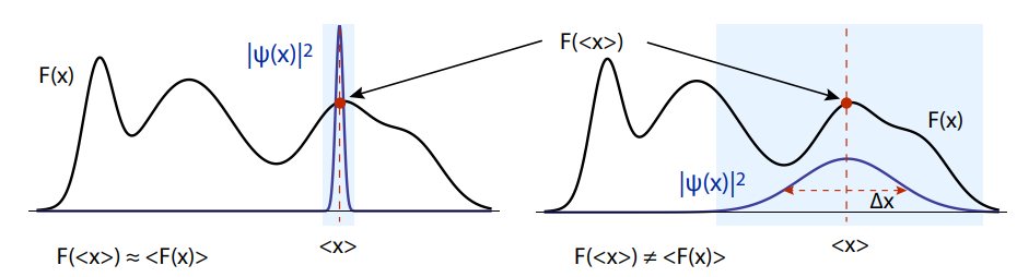
    When is the approximation above valid? We want \(\left\langle\frac{\partial V(x)}{\partial x}\right\rangle \approx \frac{\partial V(\langle x\rangle)}{\partial\langle x\rangle}\). This means that the wavefunction is localized enough such that the width of the position probability distribution is small compared to the typical length scale over which the potential varies. When this condition is satisfied, then the expectation values of quantum-mechanical probability observable will follow a classical trajectory.

    Assume for example \(\psi(x) \) is an eigenstate of the position operator \( \psi(x)=\delta(x-\bar{x})\). Then \( \langle\hat{x}\rangle=\int d x \ x \delta(x-\bar{x})^{2}=\bar{x}\) and

    \[\left\langle\frac{\partial V(x)}{\partial x}\right\rangle=\int \frac{\partial V(x)}{\partial x} \delta(x-\langle x\rangle) d x=\frac{\partial V(\langle x\rangle)}{\partial\langle x\rangle} \nonumber\]

    If instead the wavefunction is a packet centered around \( \langle x\rangle\) but with a finite width \(\Delta x \) (i.e. a Gaussian function) we no longer have an equality but only an approximation if \( \Delta x \ll L=\left|\frac{1}{V} \frac{\partial V(x)}{\partial x}\right|^{-1}\) (or localized wavefunction).


    This page titled 6.3: Evolution of Operators and Expectation Values is shared under a CC BY-NC-SA 4.0 license and was authored, remixed, and/or curated by Paola Cappellaro (MIT OpenCourseWare) via source content that was edited to the style and standards of the LibreTexts platform; a detailed edit history is available upon request.