1.3: Radioactive decay

Radioactive decay is the process in which an unstable nucleus spontaneously loses energy by emitting ionizing particles and radiation. This decay, or loss of energy, results in an atom of one type, called the parent nuclide, transforming to an atom of a different type, named the daughter nuclide.

The three principal modes of decay are called the alpha, beta and gamma decays. We will study their differences and exact mechanisms later in the class. However these decay modes share some common feature that we describe now. What these radioactive decays describe are fundamentally quantum processes, i.e. transitions among two quantum states. Thus, the radioactive decay is statistical in nature, and we can only describe the evolution of the expectation values of quantities of interest, for example the number of atoms that decay per unit time. If we observe a single unstable nucleus, we cannot know a priori when it will decay to its daughter nuclide. The time at which the decay happens is random, thus at each instant we can have the parent nuclide with some probability p and the daughter with probability 1 − p. This stochastic process can only be described in terms of the quantum mechanical evolution of the nucleus. However, if we look at an ensemble of nuclei, we can predict at each instant the average number of parent an daughter nuclides.

If we call the number of radioactive nuclei N, the number of decaying atoms per unit time is dN/dt. It is found that this rate is constant in time and it is proportional to the number of nuclei themselves:

\[\boxed{ \frac{d N}{d t}=-\lambda N(t)} \nonumber\]

The constant of proportionality λ is called the decay constant. We can also rewrite the above equation as

\[\lambda=-\frac{d N / d t}{N} \nonumber\]

where the RHS is the probability per unit time for one atom to decay. The fact that this probability is a constant is a characteristic of all radioactive decay. It also leads to the exponential law of radioactive decay:

\[N(t)=N(0) e^{-\lambda t} \nonumber\]

We can also define the mean lifetime

\[\boxed{\tau=1 / \lambda} \nonumber\]

and the half-life

\[\boxed{t_{1 / 2}=\ln (2) / \lambda} \nonumber\]

which is the time it takes for half of the atoms to decay, and the activity

\[\mathcal{A}(t)=\lambda N(t) \nonumber\]

Since \( \mathcal{A}\) can also be obtained as \(\left|\frac{d N}{d t}\right|\), the activity can be estimated from the number of decays ΔN during a small time δt such that \(\delta t \ll t_{1 / 2}\).

A common situation occurs when the daughter nuclide is also radioactive. Then we have a chain of radioactive decays, each governed by their decay laws. For example, in a chain \(N_{1} \rightarrow N_{2} \rightarrow N_{3}\), the decay of N₁ and N₂ is given by:

\[d N_{1}=-\lambda_{1} N_{1} d t, \quad d N_{2}=+\lambda_{1} N_{1} d t-\lambda_{2} N_{2} d t \nonumber\]

Another common characteristic of radioactive decays is that they are a way for unstable nuclei to reach a more energetically favorable (hence stable) configuration. In α and β decays, a nucleus emits a α or β particle, trying to approach the most stable nuclide, while in the γ decay an excited state decays toward the ground state without changing nuclear species.

Alpha decay

If we go back to the binding energy per mass number plot (B/A vs. A) we see that there is a bump (a peak) for A ∼ 60 − 100. This means that there is a corresponding minimum (or energy optimum) around these numbers. Then the heavier nuclei will want to decay toward this lighter nuclides, by shedding some protons and neutrons. More specifically, the decrease in binding energy at high A is due to Coulomb repulsion. Coulomb repulsion grows in fact as Z², much faster than the nuclear force which is ∝ A.

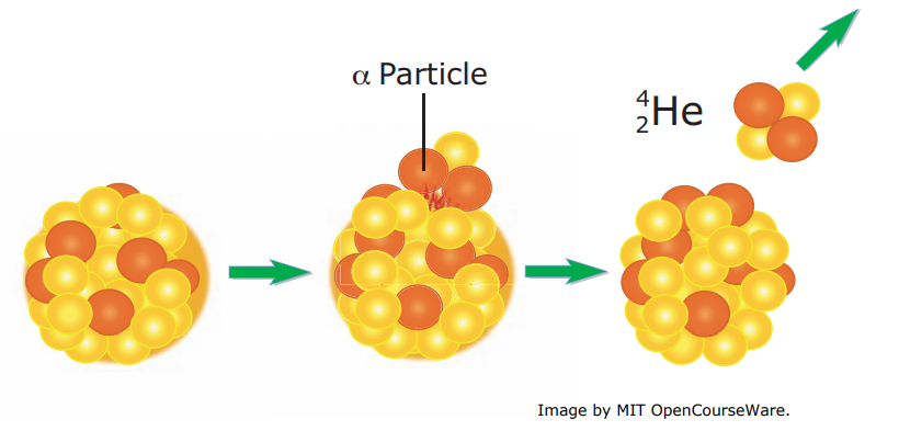
This could be thought as a similar process to what happens in the fission process: from a parent nuclide, two daughter nuclides are created. In the α decay we have specifically:

\[{ }_{Z}^{A} X_{N} \longrightarrow{ }_{Z-2}^{A-4} X_{N-2}^{\prime}+\alpha \nonumber\]

where α is the nucleus of He-4: \({ }_{2}^{4} \mathrm{He}_{2}\).

The α decay should be competing with other processes, such as the fission into equal daughter nuclides, or into pairs including ¹²C and ¹⁶O that have larger B/A then α. However α decay is usually favored. In order to understand this, we start by looking at the energetic of the decay, but we will need to study the quantum origin of the decay to arrive at a full explanation.

Figure \(\PageIndex{1}\): Alpha decay schematics. (CC BY-NC-ND; Paola Cappellaro)

Energetics

In analyzing a radioactive decay (or any nuclear reaction) an important quantity is Q, the net energy released in the decay: \(Q=\left(m_{X}-m_{X^{\prime}}-m_{\alpha}\right) c^{2} \). This is also equal to the total kinetic energy of the fragments, here \( Q=T_{X^{\prime}}+T_{\alpha}\) (here assuming that the parent nuclide is at rest).

When Q > 0 energy is released in the nuclear reaction, while for Q < 0 we need to provide energy to make the reaction happen. As in chemistry, we expect the first reaction to be a spontaneous reaction, while the second one does not happen in nature without intervention. (The first reaction is exo-energetic the second endo-energetic). Notice that it’s no coincidence that it’s called Q. In practice given some reagents and products, Q give the quality of the reaction, i.e. how energetically favorable, hence probable, it is. For example in the alpha-decay \(\log \left(t_{1 / 2}\right) \propto \frac{1}{\sqrt{Q_{\alpha}}} \), which is the Geiger-Nuttall rule (1928).

The alpha particle carries away most of the kinetic energy (since it is much lighter) and by measuring this kinetic energy experimentally it is possible to know the masses of unstable nuclides. We can calculate Q using the SEMF. Then:

\[Q_{\alpha}=B\left(\begin{array}{c} {}^{A-4}_{Z-2} \end{array} X_{N-2}^{\prime}\right)+B\left({ }^{4} H e\right)-B\left({ }_{Z}^{A} X_{N}\right)=B(A-4, Z-2)-B(A, Z)+B\left({ }^{4} H e\right) \nonumber\]

We can approximate the finite difference with the relevant gradient:

\[\begin{array}{c}
Q_{\alpha}=[B(A-4, Z-2)-B(A, Z-2)]+[B(A, Z-2)-B(A, Z)]+B\left({ }^{4} H e\right) \approx=-4 \frac{\partial B}{\partial A}-2 \frac{\partial B}{\partial Z}+B\left({ }^{4} H e\right) \\
\quad=28.3-4 a_{v}+\frac{8}{3} a_{s} A^{-1 / 3}+4 a_{c}\left(1-\frac{Z}{3 A}\right)\left(\frac{Z}{A^{1 / 3}}\right)-4 a_{\text {sym}}\left(1-\frac{2 Z}{A}+3 a_{p} A^{-7 / 4}\right)^{2}
\end{array} \nonumber\]

Since we are looking at heavy nuclei, we know that Z ≈ 0.41A (instead of Z ≈ A/2) and we obtain

\[Q_{\alpha} \approx-36.68+44.9 A^{-1 / 3}+1.02 A^{2 / 3}, \nonumber\]

where the second term comes from the surface contribution and the last term is the Coulomb term (we neglect the pairing term, since a priori we do not know if a_p is zero or not).

Then, the Coulomb term, although small, makes Q increase at large A. We find that Q ≥ 0 for \(A \gtrsim 150\), and it is Q ≈ 6MeV for A = 200. Although Q > 0, we find experimentally that α decay only arise for A ≥ 200.

Further, take for example Francium-200 \(\left(\begin{array}{ll} {}^{200}_{87} \end{array} \operatorname{Fr}_{113}\right)\). If we calculate \(Q_{\alpha}\) from the experimentally found mass differences we obtain \( Q_{\alpha} \approx 7.6 \mathrm{MeV}\) (the product is ¹⁹⁶At.) We can do the same calculation for the hypothetical decay into a ¹²C and remaining fragment \(\left(\begin{array}{l} {}^{188}_{81} \end{array} \mathrm{Tl}_{107}\right)\):

\[Q_{{}^{12}C}=c^{2}\left[m\left(\begin{array}{c} {}^{A}_{Z} \end{array} X_{N}\right)-m\left(\begin{array}{c} {}^{A-12}_{Z-6} \end{array} X_{N-6}^{\prime}\right)-m\left({ }^{12} C\right)\right] \approx 28 M e V \nonumber\]

Thus this second reaction seems to be more energetic, hence more favorable than the alpha-decay, yet it does not occur (some decays involving C-12 have been observed, but their branching ratios are much smaller).

Thus, looking only at the energetic of the decay does not explain some questions that surround the alpha decay:

• Why there’s no ¹²C-decay? (or to some of this tightly bound nuclides, e.g O-16 etc.)
• Why there’s no spontaneous fission into equal daughters?
• Why there’s alpha decay only for A ≥ 200?
• What is the explanation of Geiger-Nuttall rule? \( \log t_{1 / 2} \propto \frac{1}{\sqrt{Q_{\alpha}}}\)

Beta decay

The beta decay is a radioactive decay in which a proton in a nucleus is converted into a neutron (or vice-versa). Thus A is constant, but Z and N change by 1. In the process the nucleus emits a beta particle (either an electron or a positron) and quasi-massless particle, the neutrino

Figure \(\PageIndex{2}\): Beta decay schematics (CC BY-NC-ND; Paola Cappellaro)

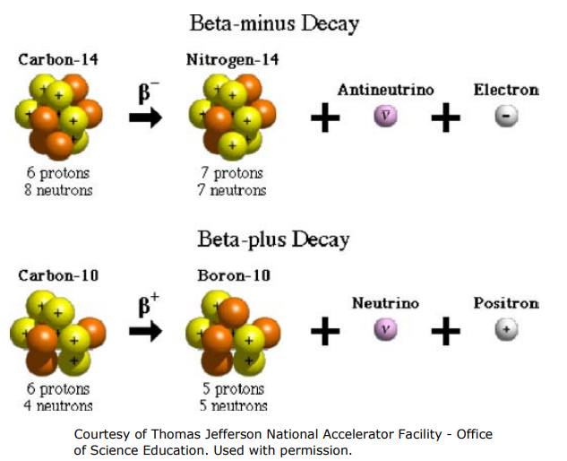
There are 3 types of beta decay:

\[{ }_{Z}^{A} X_{N} \rightarrow{ }_{Z+1}^{A} X_{N-1}^{\prime}+e^{-}+\bar{\nu} \nonumber\]

This is the \(\beta^{-} \) decay (or negative beta decay). The underlying reaction is:

\[n \rightarrow p+e^{-}+\bar{\nu} \nonumber\]

that corresponds to the conversion of a proton into a neutron with the emission of an electron and an anti-neutrino. There are two other types of reactions, the \( \beta^{+}\) reaction,

\[{}^{A}_{Z} X_{N} \rightarrow{ }_{Z-1}^{A} X_{N+1}^{\prime}+e^{+}+\nu \quad \Longleftrightarrow \quad p \rightarrow n+e^{+}+\nu \nonumber\]

which sees the emission of a positron (the electron anti-particle) and a neutrino; and the electron capture:

\[{}^{A}_{Z} X_{N}+e^{-} \rightarrow{ }_{Z-1}^{A} X_{N+1}^{\prime}+\nu \quad \Longleftrightarrow \quad p+e^{-} \rightarrow n+\nu \nonumber\]

a process that competes with, or substitutes, the positron emission.

Recall the mass of nuclide as given by the semi-empirical mass formula. If we keep A fixed, the SEMF gives the binding energy as a function of Z. The only term that depends explicitly on Z is the Coulomb term. By inspection we see that B ∝ Z². Then from the SEMF we have that the masses of possible nuclides with the same mass number lie on a parabola. Nuclides lower in the parabola have smaller M and are thus more stable. In order to reach that minimum, unstable nuclides undergo a decay process to transform excess protons in neutrons (and vice-versa).

Figure \(\PageIndex{3}\): Nuclear Mass Chain for A=125, (left) and A=128 (right). (CC BY-NC-ND; Paola Cappellaro)

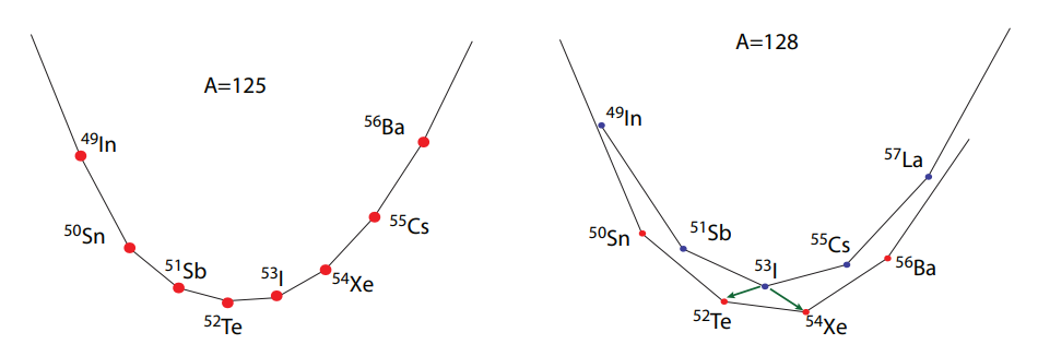
The beta decay is the radioactive decay process that can convert protons into neutrons (and vice-versa). We will study more in depth this mechanism, but here we want simply to point out how this process can be energetically favorable, and thus we can predict which transitions are likely to occur, based only on the SEMF.

For example, for A = 125 if Z < 52 we have a favorable n → p conversion (beta decay) while for Z > 52 we have p → n (or positron beta decay), so that the stable nuclide is Z = 52 (tellurium).

Conservation laws

As the neutrino is hard to detect, initially the beta decay seemed to violate energy conservation. Introducing an extra particle in the process allows one to respect conservation of energy.

The Q value of a beta decay is given by the usual formula:

\[Q_{\beta^{-}}=\left[m_{N}\left({ }^{A} X\right)-m_{N}\left({ }_{Z+1}^{A} X^{\prime}\right)-m_{e}\right] c^{2} . \nonumber\]

Using the atomic masses and neglecting the electron’s binding energies as usual we have

\[Q_{\beta^{-}}=\left\{\left[m_{A}\left({ }^{A} X\right)-Z m_{e}\right]-\left[m_{A}\left({ }_{Z+1}^{A} X^{\prime}\right)-(Z+1) m_{e}\right]-m_{e}\right\} c^{2}=\left[m_{A}\left({ }^{A} X\right)-m_{A}\left({ }_{Z+1}^{A} X^{\prime}\right)\right] c^{2}. \nonumber\]

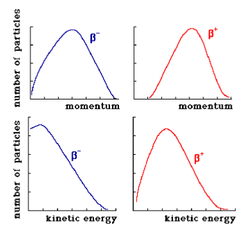
The kinetic energy (equal to the Q) is shared by the neutrino and the electron (we neglect any recoil of the massive nucleus). Then, the emerging electron (remember, the only particle that we can really observe) does not have a fixed energy, as it was for example for the gamma photon. But it will exhibit a spectrum of energy (or the number of electron at a given energy) as well as a distribution of momenta. We will see how we can reproduce these plots by analyzing the QM theory of beta decay.

Examples

\[ { }_{29}^{64} \mathrm{Cu}_{\searrow}^{\nearrow} \begin{array}{cc} { }_{30}^{64} \mathrm{Zn}+e^{-}+\bar{\nu}, & Q_{\beta}=0.57 \ \mathrm{MeV} \\ { }_{28}^{64} \mathrm{Ni}+e^{+}+\nu, & Q_{\beta}=0.66 \ \mathrm{MeV} \end{array} \nonumber\]

The neutrino and beta particle (\(\beta^{\pm}\)) share the energy. Since the neutrinos are very difficult to detect (as we will see they are almost massless and interact very weakly with matter), the electrons/positrons are the particles detected in beta-decay and they present a characteristic energy spectrum (see Fig. \(\PageIndex{4}\)).

The difference between the spectrum of the \(\beta^{\pm}\) particles is due to the Coulomb repulsion or attraction from the nucleus.

© Neil Spooner. All rights reserved. This content is excluded from our Creative Commons license. For more information, see http://ocw.mit.edu/fairuse.

Figure \(\PageIndex{4}\): Beta decay spectra: Distribution of momentum (top plots) and kinetic energy (bottom) for \(\beta^{-}\) (left) and \(\beta^{+}\) (right) decay.

Notice that the neutrinos also carry away angular momentum. They are spin-1/2 particles, with no charge (hence the name) and very small mass. For many years it was actually believed to have zero mass. However it has been confirmed that it does have a mass in 1998.

Other conserved quantities are:

• Momentum: The momentum is also shared between the electron and the neutrino. Thus the observed electron momentum ranges from zero to a maximum possible momentum transfer.
• Angular momentum (both the electron and the neutrino have spin 1/2)
• Parity? It turns out that parity is not conserved in this decay. This hints to the fact that the interaction responsible violates parity conservation (so it cannot be the same interactions we already studies, e.m. and strong interactions)
• Charge (thus the creation of a proton is for example always accompanied by the creation of an electron)
• Lepton number: we do not conserve the total number of particles (we create beta and neutrinos). However the number of massive, heavy particles (or baryons, composed of 3 quarks) is conserved. Also the lepton number is conserved. Leptons are fundamental particles (including the electron, muon and tau, as well as the three types of neutrinos associated with these 3). The lepton number is +1 for these particles and -1 for their antiparticles. Then an electron is always accompanied by the creation of an antineutrino, e.g., to conserve the lepton number (initially zero).

Although the energy involved in the decay can predict whether a beta decay will occur (Q > 0), and which type of beta decay does occur, the decay rate can be quite different even for similar Q-values. Consider for example \({ }^{22} \mathrm{Na}\) and \({ }^{36} \mathrm{Cl}\). They both decay by \( \beta\) decay:

\[{ }_{11}^{22} \mathrm{Na}_{11} \rightarrow_{10}^{22} \mathrm{Ne}_{12}+\beta^{+}+\nu, \quad Q=0.22 \mathrm{MeV}, \quad T_{\frac{1}{2}}=2.6 \text { years } \nonumber\]

\[{ }_{17}^{36} \mathrm{Cl}_{19} \rightarrow_{18}^{36} \mathrm{Ar}_{18}+\beta^{-}+\bar{\nu} \quad Q=0.25 \mathrm{MeV}, \quad T_{\frac{1}{2}}=3 \times 10^{5} \text { years } \nonumber\]

Even if they have very close Q-values, there is a five order magnitude in the lifetime. Thus we need to look closer to the nuclear structure in order to understand these differences.

Gamma decay

In the gamma decay the nuclide is unchanged, but it goes from an excited to a lower energy state. These states are called isomeric states. Usually the reaction is written as:

\[{ }_{Z}^{A} X_{N}^{*} \longrightarrow{ }_{Z}^{A} X_{N}+\gamma \nonumber\]

where the star indicate an excited state. We will study that the gamma energy depends on the energy difference between these two states, but which decays can happen depend, once again, on the details of the nuclear structure and on quantum-mechanical selection rules associated with the nuclear angular momentum.

Spontaneous fission

Some nuclei can spontaneously undergo a fission, even outside the particular conditions found in a nuclear reactor. In the process a heavy nuclide splits into two lighter nuclei, of roughly the same mass.

Branching Ratios

Some nuclei only decay via a single process, but sometimes they can undergo many different radioactive processes, that compete one with the other. The relative intensities of the competing decays are called branching ratios.

Branching ratios are expressed as percentage or sometimes as partial half-lives. For example, if a nucleus can decay by beta decay (and other modes) with a branching ration \(b_{\beta}\) the partial half-life for the beta decay is \(\lambda_{\beta}=b_{\beta} \lambda\).