Physics LibreTexts

8.3: The quark model of strong interactions

  • Page ID
    15047
  • \( \newcommand{\vecs}[1]{\overset { \scriptstyle \rightharpoonup} {\mathbf{#1}} } \)

    \( \newcommand{\vecd}[1]{\overset{-\!-\!\rightharpoonup}{\vphantom{a}\smash {#1}}} \)

    \( \newcommand{\dsum}{\displaystyle\sum\limits} \)

    \( \newcommand{\dint}{\displaystyle\int\limits} \)

    \( \newcommand{\dlim}{\displaystyle\lim\limits} \)

    \( \newcommand{\id}{\mathrm{id}}\) \( \newcommand{\Span}{\mathrm{span}}\)

    ( \newcommand{\kernel}{\mathrm{null}\,}\) \( \newcommand{\range}{\mathrm{range}\,}\)

    \( \newcommand{\RealPart}{\mathrm{Re}}\) \( \newcommand{\ImaginaryPart}{\mathrm{Im}}\)

    \( \newcommand{\Argument}{\mathrm{Arg}}\) \( \newcommand{\norm}[1]{\| #1 \|}\)

    \( \newcommand{\inner}[2]{\langle #1, #2 \rangle}\)

    \( \newcommand{\Span}{\mathrm{span}}\)

    \( \newcommand{\id}{\mathrm{id}}\)

    \( \newcommand{\Span}{\mathrm{span}}\)

    \( \newcommand{\kernel}{\mathrm{null}\,}\)

    \( \newcommand{\range}{\mathrm{range}\,}\)

    \( \newcommand{\RealPart}{\mathrm{Re}}\)

    \( \newcommand{\ImaginaryPart}{\mathrm{Im}}\)

    \( \newcommand{\Argument}{\mathrm{Arg}}\)

    \( \newcommand{\norm}[1]{\| #1 \|}\)

    \( \newcommand{\inner}[2]{\langle #1, #2 \rangle}\)

    \( \newcommand{\Span}{\mathrm{span}}\) \( \newcommand{\AA}{\unicode[.8,0]{x212B}}\)

    \( \newcommand{\vectorA}[1]{\vec{#1}}      % arrow\)

    \( \newcommand{\vectorAt}[1]{\vec{\text{#1}}}      % arrow\)

    \( \newcommand{\vectorB}[1]{\overset { \scriptstyle \rightharpoonup} {\mathbf{#1}} } \)

    \( \newcommand{\vectorC}[1]{\textbf{#1}} \)

    \( \newcommand{\vectorD}[1]{\overrightarrow{#1}} \)

    \( \newcommand{\vectorDt}[1]{\overrightarrow{\text{#1}}} \)

    \( \newcommand{\vectE}[1]{\overset{-\!-\!\rightharpoonup}{\vphantom{a}\smash{\mathbf {#1}}}} \)

    \( \newcommand{\vecs}[1]{\overset { \scriptstyle \rightharpoonup} {\mathbf{#1}} } \)

    \(\newcommand{\longvect}{\overrightarrow}\)

    \( \newcommand{\vecd}[1]{\overset{-\!-\!\rightharpoonup}{\vphantom{a}\smash {#1}}} \)

    \(\newcommand{\avec}{\mathbf a}\) \(\newcommand{\bvec}{\mathbf b}\) \(\newcommand{\cvec}{\mathbf c}\) \(\newcommand{\dvec}{\mathbf d}\) \(\newcommand{\dtil}{\widetilde{\mathbf d}}\) \(\newcommand{\evec}{\mathbf e}\) \(\newcommand{\fvec}{\mathbf f}\) \(\newcommand{\nvec}{\mathbf n}\) \(\newcommand{\pvec}{\mathbf p}\) \(\newcommand{\qvec}{\mathbf q}\) \(\newcommand{\svec}{\mathbf s}\) \(\newcommand{\tvec}{\mathbf t}\) \(\newcommand{\uvec}{\mathbf u}\) \(\newcommand{\vvec}{\mathbf v}\) \(\newcommand{\wvec}{\mathbf w}\) \(\newcommand{\xvec}{\mathbf x}\) \(\newcommand{\yvec}{\mathbf y}\) \(\newcommand{\zvec}{\mathbf z}\) \(\newcommand{\rvec}{\mathbf r}\) \(\newcommand{\mvec}{\mathbf m}\) \(\newcommand{\zerovec}{\mathbf 0}\) \(\newcommand{\onevec}{\mathbf 1}\) \(\newcommand{\real}{\mathbb R}\) \(\newcommand{\twovec}[2]{\left[\begin{array}{r}#1 \\ #2 \end{array}\right]}\) \(\newcommand{\ctwovec}[2]{\left[\begin{array}{c}#1 \\ #2 \end{array}\right]}\) \(\newcommand{\threevec}[3]{\left[\begin{array}{r}#1 \\ #2 \\ #3 \end{array}\right]}\) \(\newcommand{\cthreevec}[3]{\left[\begin{array}{c}#1 \\ #2 \\ #3 \end{array}\right]}\) \(\newcommand{\fourvec}[4]{\left[\begin{array}{r}#1 \\ #2 \\ #3 \\ #4 \end{array}\right]}\) \(\newcommand{\cfourvec}[4]{\left[\begin{array}{c}#1 \\ #2 \\ #3 \\ #4 \end{array}\right]}\) \(\newcommand{\fivevec}[5]{\left[\begin{array}{r}#1 \\ #2 \\ #3 \\ #4 \\ #5 \\ \end{array}\right]}\) \(\newcommand{\cfivevec}[5]{\left[\begin{array}{c}#1 \\ #2 \\ #3 \\ #4 \\ #5 \\ \end{array}\right]}\) \(\newcommand{\mattwo}[4]{\left[\begin{array}{rr}#1 \amp #2 \\ #3 \amp #4 \\ \end{array}\right]}\) \(\newcommand{\laspan}[1]{\text{Span}\{#1\}}\) \(\newcommand{\bcal}{\cal B}\) \(\newcommand{\ccal}{\cal C}\) \(\newcommand{\scal}{\cal S}\) \(\newcommand{\wcal}{\cal W}\) \(\newcommand{\ecal}{\cal E}\) \(\newcommand{\coords}[2]{\left\{#1\right\}_{#2}}\) \(\newcommand{\gray}[1]{\color{gray}{#1}}\) \(\newcommand{\lgray}[1]{\color{lightgray}{#1}}\) \(\newcommand{\rank}{\operatorname{rank}}\) \(\newcommand{\row}{\text{Row}}\) \(\newcommand{\col}{\text{Col}}\) \(\renewcommand{\row}{\text{Row}}\) \(\newcommand{\nul}{\text{Nul}}\) \(\newcommand{\var}{\text{Var}}\) \(\newcommand{\corr}{\text{corr}}\) \(\newcommand{\len}[1]{\left|#1\right|}\) \(\newcommand{\bbar}{\overline{\bvec}}\) \(\newcommand{\bhat}{\widehat{\bvec}}\) \(\newcommand{\bperp}{\bvec^\perp}\) \(\newcommand{\xhat}{\widehat{\xvec}}\) \(\newcommand{\vhat}{\widehat{\vvec}}\) \(\newcommand{\uhat}{\widehat{\uvec}}\) \(\newcommand{\what}{\widehat{\wvec}}\) \(\newcommand{\Sighat}{\widehat{\Sigma}}\) \(\newcommand{\lt}{<}\) \(\newcommand{\gt}{>}\) \(\newcommand{\amp}{&}\) \(\definecolor{fillinmathshade}{gray}{0.9}\)

    Once the eightfold way (as the SU(3) symmetry was poetically referred to) was discovered, the race was on to explain it. As I have shown before the decaplet and two octets occur in the product \[{\mathbf{3}} \otimes {\mathbf{3}} \otimes {\mathbf{3}} = {\mathbf{1}} \oplus {\mathbf{8} }\oplus {\mathbf{8}} \oplus{\mathbf{10}}. \nonumber \] A very natural assumption is to introduce a new particle that comes in three “flavours” called up, down and strange (\(u\), \(d\) and \(s\), respectively), and assume that the baryons are made from three of such particles, and the mesons from a quark and anti-quark (remember,| =.) Each of these quarks carries one third a unit of baryon number. The properties can now be tabulated (Table \(\PageIndex{1}\)).

    Table \(\PageIndex{1}\): The properties of the three quarks.
    Quark label spin \(Q/e\) \(I\) \(I_3\) \(S\) \(B\)
    Up \(u\) \(\frac{1}{2}\) \(+\frac{2}{3}\) \(\frac{1}{2}\) +\(\frac{1}{2}\) 0 \(\frac{1}{3}\)
    Down \(d\) \(\frac{1}{2}\) \(-\frac{1}{3}\) \(\frac{1}{2}\) -\(\frac{1}{2}\) 0 \(\frac{1}{3}\)
    Strange \(s\) \(\frac{1}{2}\) \(-\frac{1}{3}\) \(0\) \(0\) -1 \(\frac{1}{3}\)

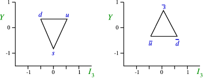
    In the multiplet language I used before, we find that the quarks form a triangle, as given in Figure \(\PageIndex{1}\).

    Two graphs show shapes: a trapezoid labeled \(d\) and \(s\) on the left, and a triangle labeled \(2\), \(p\), and \(3\) on the right.
    Figure \(\PageIndex{1}\): The multiplet structure of quarks and antiquarks

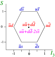
    Once we have made this assignment, we can try to derive what combination corresponds to the assignments of the meson octet, Figure \(\PageIndex{2}\). We just make all possible combinations of a quark and antiquark, apart from the scalar one \(\eta'=u\bar{u}+d\bar{d} +c\bar{c}\) (why?).

    A hexagonal plot showing particle states labeled with colors: red, blue, and purple points representing quark combinations for S versus I3.
    Figure \(\PageIndex{2}\): quark assignment of the meson octet

    A similar assignment can be made for the nucleon octet, and the nucleon decaplet, see e.g., see FFigure \(\PageIndex{3}\).

    A hexagonal graph showing coordinates labeled with quark combinations, positioned in the I3-Y plane.
    Figure \(\PageIndex{3}\): quark assignment of the nucleon octet

    This page titled 8.3: The quark model of strong interactions is shared under a CC BY-NC-SA 2.0 license and was authored, remixed, and/or curated by Niels Walet via source content that was edited to the style and standards of the LibreTexts platform.